1 🏁 Computational Foundations 🏗️ for Strategic Business Analytics

Author

Stefan Edlinger-Bach, PhD

1.1 Learning Objectives

By the end of this chapter, you will be able to:

Set up and navigate the R and RStudio environment
Understand the core principles of the Tidyverse ecosystem
Import and export data in various formats
Transform and manipulate data using dplyr
Create and modify variables
Filter, arrange, and summarize data
Perform group-wise operations
Join multiple datasets
Handle missing data and outliers
Apply functions to data using iteration

1.2 Prerequisites

For this chapter, you’ll need:

R and RStudio installed on your computer
Basic understanding of programming concepts (variables, functions, etc.)
The following R packages installed:

# Install required packages if not already installed
if (!require("tidyverse")) install.packages("tidyverse")
if (!require("readxl")) install.packages("readxl")
if (!require("haven")) install.packages("haven")
if (!require("janitor")) install.packages("janitor")
if (!require("skimr")) install.packages("skimr")
if (!require("lubridate")) install.packages("lubridate")
if (!require("scales")) install.packages("scales")

# Load required packages
library(tidyverse)      # For data manipulation and visualization
library(readxl)         # For reading Excel files
library(haven)          # For reading SPSS, SAS, and Stata files
library(janitor)        # For cleaning data
library(skimr)          # For data summaries
library(lubridate)      # For date manipulation
library(scales)         # For formatting numbers and dates

1.3 Introduction to R and RStudio

R is a powerful programming language and environment for statistical computing and graphics. RStudio is an integrated development environment (IDE) that makes working with R easier and more productive.

Why R for Business Analytics?

R has several advantages for business analytics:

Open Source: Free to use and continuously improved by a large community
Comprehensive: Thousands of packages for various analytical tasks
Reproducible: Code-based approach ensures reproducibility
Flexible: Can handle various data formats and analytical methods
Visualization: Powerful tools for creating high-quality visualizations
Integration: Can integrate with other tools and languages

RStudio Interface

The RStudio interface consists of four main panes:

Source Editor: Where you write and edit your R code
Console: Where you execute R commands and see the results
Environment/History: Shows your current variables and command history
Files/Plots/Packages/Help: Shows files, plots, installed packages, and help documentation

R Basics

Let’s start with some basic R operations:

# Basic arithmetic
5 + 3

[1] 8

10 - 2

[1] 8

4 * 5

[1] 20

20 / 4

[1] 5

2^3  # Exponentiation

[1] 8

# Variables
x <- 10  # Assignment
y <- 5
x + y

[1] 15

# Functions
sqrt(25)

[1] 5

log(10)

[1] 2.302585

round(3.14159, 2)

[1] 3.14

# Vectors
numbers <- c(1, 2, 3, 4, 5)
numbers * 2

[1]  2  4  6  8 10

sum(numbers)

[1] 15

mean(numbers)

[1] 3

# Character vectors
fruits <- c("apple", "banana", "orange")
paste("I like", fruits)

[1] "I like apple"  "I like banana" "I like orange"

# Logical vectors
is_even <- numbers %% 2 == 0
numbers[is_even]

[1] 2 4

1.4 Introduction to the Tidyverse

The Tidyverse is a collection of R packages designed for data science. These packages share a common philosophy and are designed to work together seamlessly.

Core Tidyverse Packages

dplyr: For data manipulation
tidyr: For tidying data
readr: For reading rectangular data
ggplot2: For data visualization
purrr: For functional programming
tibble: For modern data frames
stringr: For string manipulation
forcats: For working with factors

Tidy Data Principles

Tidy data is a standard way of organizing data where:

Each variable forms a column
Each observation forms a row
Each type of observational unit forms a table

# Example of tidy data
tidy_data <- tibble(
  country = c("USA", "USA", "Canada", "Canada"),
  year = c(2020, 2021, 2020, 2021),
  gdp = c(20.94, 22.99, 1.64, 1.99)
)

tidy_data

# A tibble: 4 × 3
  country  year   gdp
  <chr>   <dbl> <dbl>
1 USA      2020 20.9 
2 USA      2021 23.0 
3 Canada   2020  1.64
4 Canada   2021  1.99

1.5 Importing Data

R can import data from various sources and formats.

Reading CSV Files

# Create a sample CSV file
write.csv(
  data.frame(
    ID = 1:5,
    Name = c("Alice", "Bob", "Charlie", "David", "Eve"),
    Sales = c(120, 340, 260, 180, 420)
  ),
  "sample_data.csv",
  row.names = FALSE
)

# Read the CSV file
sales_data <- read_csv("sample_data.csv")

Rows: 5 Columns: 3
── Column specification ────────────────────────────────────────────────────────
Delimiter: ","
chr (1): Name
dbl (2): ID, Sales

ℹ Use `spec()` to retrieve the full column specification for this data.
ℹ Specify the column types or set `show_col_types = FALSE` to quiet this message.

sales_data

# A tibble: 5 × 3
     ID Name    Sales
  <dbl> <chr>   <dbl>
1     1 Alice     120
2     2 Bob       340
3     3 Charlie   260
4     4 David     180
5     5 Eve       420

Reading Excel Files

# Read an Excel file
# excel_data <- read_excel("sample_data.xlsx", sheet = "Sheet1")

Reading Other Formats

# Read SPSS file
# spss_data <- read_spss("sample_data.sav")

# Read SAS file
# sas_data <- read_sas("sample_data.sas7bdat")

# Read Stata file
# stata_data <- read_stata("sample_data.dta")

# Read RDS file (R's native format)
# rds_data <- readRDS("sample_data.rds")

Reading Data from Databases

# Using the DBI package to connect to databases
# library(DBI)
# library(RSQLite)

# Connect to a SQLite database
# con <- dbConnect(SQLite(), "sample_database.sqlite")

# Read data from a table
# db_data <- dbReadTable(con, "sales")

# Execute a SQL query
# query_data <- dbGetQuery(con, "SELECT * FROM sales WHERE Sales > 200")

# Disconnect from the database
# dbDisconnect(con)

1.6 Data Transformation with dplyr

dplyr is a grammar of data manipulation, providing a consistent set of verbs that help you solve the most common data manipulation challenges.

The Five Main dplyr Verbs

select(): Select columns
filter(): Filter rows
arrange(): Reorder rows
mutate(): Create new variables
summarize(): Summarize data

Let’s use a built-in dataset to demonstrate these verbs:

# Load the built-in mtcars dataset
data(mtcars)

# Convert to a tibble for better printing
cars <- as_tibble(mtcars, rownames = "model")
cars

# A tibble: 32 × 12
   model         mpg   cyl  disp    hp  drat    wt  qsec    vs    am  gear  carb
   <chr>       <dbl> <dbl> <dbl> <dbl> <dbl> <dbl> <dbl> <dbl> <dbl> <dbl> <dbl>
 1 Mazda RX4    21       6  160    110  3.9   2.62  16.5     0     1     4     4
 2 Mazda RX4 …  21       6  160    110  3.9   2.88  17.0     0     1     4     4
 3 Datsun 710   22.8     4  108     93  3.85  2.32  18.6     1     1     4     1
 4 Hornet 4 D…  21.4     6  258    110  3.08  3.22  19.4     1     0     3     1
 5 Hornet Spo…  18.7     8  360    175  3.15  3.44  17.0     0     0     3     2
 6 Valiant      18.1     6  225    105  2.76  3.46  20.2     1     0     3     1
 7 Duster 360   14.3     8  360    245  3.21  3.57  15.8     0     0     3     4
 8 Merc 240D    24.4     4  147.    62  3.69  3.19  20       1     0     4     2
 9 Merc 230     22.8     4  141.    95  3.92  3.15  22.9     1     0     4     2
10 Merc 280     19.2     6  168.   123  3.92  3.44  18.3     1     0     4     4
# ℹ 22 more rows

Selecting Columns

# Select specific columns
cars %>%
  select(model, mpg, hp, wt)

# A tibble: 32 × 4
   model               mpg    hp    wt
   <chr>             <dbl> <dbl> <dbl>
 1 Mazda RX4          21     110  2.62
 2 Mazda RX4 Wag      21     110  2.88
 3 Datsun 710         22.8    93  2.32
 4 Hornet 4 Drive     21.4   110  3.22
 5 Hornet Sportabout  18.7   175  3.44
 6 Valiant            18.1   105  3.46
 7 Duster 360         14.3   245  3.57
 8 Merc 240D          24.4    62  3.19
 9 Merc 230           22.8    95  3.15
10 Merc 280           19.2   123  3.44
# ℹ 22 more rows

# Select columns by position
cars %>%
  select(1, 2, 3, 4)

# A tibble: 32 × 4
   model               mpg   cyl  disp
   <chr>             <dbl> <dbl> <dbl>
 1 Mazda RX4          21       6  160 
 2 Mazda RX4 Wag      21       6  160 
 3 Datsun 710         22.8     4  108 
 4 Hornet 4 Drive     21.4     6  258 
 5 Hornet Sportabout  18.7     8  360 
 6 Valiant            18.1     6  225 
 7 Duster 360         14.3     8  360 
 8 Merc 240D          24.4     4  147.
 9 Merc 230           22.8     4  141.
10 Merc 280           19.2     6  168.
# ℹ 22 more rows

# Select columns by range
cars %>%
  select(model:disp)

# A tibble: 32 × 4
   model               mpg   cyl  disp
   <chr>             <dbl> <dbl> <dbl>
 1 Mazda RX4          21       6  160 
 2 Mazda RX4 Wag      21       6  160 
 3 Datsun 710         22.8     4  108 
 4 Hornet 4 Drive     21.4     6  258 
 5 Hornet Sportabout  18.7     8  360 
 6 Valiant            18.1     6  225 
 7 Duster 360         14.3     8  360 
 8 Merc 240D          24.4     4  147.
 9 Merc 230           22.8     4  141.
10 Merc 280           19.2     6  168.
# ℹ 22 more rows

# Select columns by pattern
cars %>%
  select(starts_with("c"))

# A tibble: 32 × 2
     cyl  carb
   <dbl> <dbl>
 1     6     4
 2     6     4
 3     4     1
 4     6     1
 5     8     2
 6     6     1
 7     8     4
 8     4     2
 9     4     2
10     6     4
# ℹ 22 more rows

# Exclude columns
cars %>%
  select(-carb, -vs, -am)

# A tibble: 32 × 9
   model               mpg   cyl  disp    hp  drat    wt  qsec  gear
   <chr>             <dbl> <dbl> <dbl> <dbl> <dbl> <dbl> <dbl> <dbl>
 1 Mazda RX4          21       6  160    110  3.9   2.62  16.5     4
 2 Mazda RX4 Wag      21       6  160    110  3.9   2.88  17.0     4
 3 Datsun 710         22.8     4  108     93  3.85  2.32  18.6     4
 4 Hornet 4 Drive     21.4     6  258    110  3.08  3.22  19.4     3
 5 Hornet Sportabout  18.7     8  360    175  3.15  3.44  17.0     3
 6 Valiant            18.1     6  225    105  2.76  3.46  20.2     3
 7 Duster 360         14.3     8  360    245  3.21  3.57  15.8     3
 8 Merc 240D          24.4     4  147.    62  3.69  3.19  20       4
 9 Merc 230           22.8     4  141.    95  3.92  3.15  22.9     4
10 Merc 280           19.2     6  168.   123  3.92  3.44  18.3     4
# ℹ 22 more rows

Filtering Rows

# Filter rows based on a condition
cars %>%
  filter(mpg > 20)

# A tibble: 14 × 12
   model         mpg   cyl  disp    hp  drat    wt  qsec    vs    am  gear  carb
   <chr>       <dbl> <dbl> <dbl> <dbl> <dbl> <dbl> <dbl> <dbl> <dbl> <dbl> <dbl>
 1 Mazda RX4    21       6 160     110  3.9   2.62  16.5     0     1     4     4
 2 Mazda RX4 …  21       6 160     110  3.9   2.88  17.0     0     1     4     4
 3 Datsun 710   22.8     4 108      93  3.85  2.32  18.6     1     1     4     1
 4 Hornet 4 D…  21.4     6 258     110  3.08  3.22  19.4     1     0     3     1
 5 Merc 240D    24.4     4 147.     62  3.69  3.19  20       1     0     4     2
 6 Merc 230     22.8     4 141.     95  3.92  3.15  22.9     1     0     4     2
 7 Fiat 128     32.4     4  78.7    66  4.08  2.2   19.5     1     1     4     1
 8 Honda Civic  30.4     4  75.7    52  4.93  1.62  18.5     1     1     4     2
 9 Toyota Cor…  33.9     4  71.1    65  4.22  1.84  19.9     1     1     4     1
10 Toyota Cor…  21.5     4 120.     97  3.7   2.46  20.0     1     0     3     1
11 Fiat X1-9    27.3     4  79      66  4.08  1.94  18.9     1     1     4     1
12 Porsche 91…  26       4 120.     91  4.43  2.14  16.7     0     1     5     2
13 Lotus Euro…  30.4     4  95.1   113  3.77  1.51  16.9     1     1     5     2
14 Volvo 142E   21.4     4 121     109  4.11  2.78  18.6     1     1     4     2

# Multiple conditions with AND
cars %>%
  filter(mpg > 20, hp > 100)

# A tibble: 5 × 12
  model          mpg   cyl  disp    hp  drat    wt  qsec    vs    am  gear  carb
  <chr>        <dbl> <dbl> <dbl> <dbl> <dbl> <dbl> <dbl> <dbl> <dbl> <dbl> <dbl>
1 Mazda RX4     21       6 160     110  3.9   2.62  16.5     0     1     4     4
2 Mazda RX4 W…  21       6 160     110  3.9   2.88  17.0     0     1     4     4
3 Hornet 4 Dr…  21.4     6 258     110  3.08  3.22  19.4     1     0     3     1
4 Lotus Europa  30.4     4  95.1   113  3.77  1.51  16.9     1     1     5     2
5 Volvo 142E    21.4     4 121     109  4.11  2.78  18.6     1     1     4     2

# Multiple conditions with OR
cars %>%
  filter(mpg > 30 | hp > 200)

# A tibble: 11 × 12
   model         mpg   cyl  disp    hp  drat    wt  qsec    vs    am  gear  carb
   <chr>       <dbl> <dbl> <dbl> <dbl> <dbl> <dbl> <dbl> <dbl> <dbl> <dbl> <dbl>
 1 Duster 360   14.3     8 360     245  3.21  3.57  15.8     0     0     3     4
 2 Cadillac F…  10.4     8 472     205  2.93  5.25  18.0     0     0     3     4
 3 Lincoln Co…  10.4     8 460     215  3     5.42  17.8     0     0     3     4
 4 Chrysler I…  14.7     8 440     230  3.23  5.34  17.4     0     0     3     4
 5 Fiat 128     32.4     4  78.7    66  4.08  2.2   19.5     1     1     4     1
 6 Honda Civic  30.4     4  75.7    52  4.93  1.62  18.5     1     1     4     2
 7 Toyota Cor…  33.9     4  71.1    65  4.22  1.84  19.9     1     1     4     1
 8 Camaro Z28   13.3     8 350     245  3.73  3.84  15.4     0     0     3     4
 9 Lotus Euro…  30.4     4  95.1   113  3.77  1.51  16.9     1     1     5     2
10 Ford Pante…  15.8     8 351     264  4.22  3.17  14.5     0     1     5     4
11 Maserati B…  15       8 301     335  3.54  3.57  14.6     0     1     5     8

# Filter with %in%
cars %>%
  filter(cyl %in% c(4, 6))

# A tibble: 18 × 12
   model         mpg   cyl  disp    hp  drat    wt  qsec    vs    am  gear  carb
   <chr>       <dbl> <dbl> <dbl> <dbl> <dbl> <dbl> <dbl> <dbl> <dbl> <dbl> <dbl>
 1 Mazda RX4    21       6 160     110  3.9   2.62  16.5     0     1     4     4
 2 Mazda RX4 …  21       6 160     110  3.9   2.88  17.0     0     1     4     4
 3 Datsun 710   22.8     4 108      93  3.85  2.32  18.6     1     1     4     1
 4 Hornet 4 D…  21.4     6 258     110  3.08  3.22  19.4     1     0     3     1
 5 Valiant      18.1     6 225     105  2.76  3.46  20.2     1     0     3     1
 6 Merc 240D    24.4     4 147.     62  3.69  3.19  20       1     0     4     2
 7 Merc 230     22.8     4 141.     95  3.92  3.15  22.9     1     0     4     2
 8 Merc 280     19.2     6 168.    123  3.92  3.44  18.3     1     0     4     4
 9 Merc 280C    17.8     6 168.    123  3.92  3.44  18.9     1     0     4     4
10 Fiat 128     32.4     4  78.7    66  4.08  2.2   19.5     1     1     4     1
11 Honda Civic  30.4     4  75.7    52  4.93  1.62  18.5     1     1     4     2
12 Toyota Cor…  33.9     4  71.1    65  4.22  1.84  19.9     1     1     4     1
13 Toyota Cor…  21.5     4 120.     97  3.7   2.46  20.0     1     0     3     1
14 Fiat X1-9    27.3     4  79      66  4.08  1.94  18.9     1     1     4     1
15 Porsche 91…  26       4 120.     91  4.43  2.14  16.7     0     1     5     2
16 Lotus Euro…  30.4     4  95.1   113  3.77  1.51  16.9     1     1     5     2
17 Ferrari Di…  19.7     6 145     175  3.62  2.77  15.5     0     1     5     6
18 Volvo 142E   21.4     4 121     109  4.11  2.78  18.6     1     1     4     2

# Filter with between
cars %>%
  filter(between(mpg, 15, 20))

# A tibble: 13 × 12
   model         mpg   cyl  disp    hp  drat    wt  qsec    vs    am  gear  carb
   <chr>       <dbl> <dbl> <dbl> <dbl> <dbl> <dbl> <dbl> <dbl> <dbl> <dbl> <dbl>
 1 Hornet Spo…  18.7     8  360    175  3.15  3.44  17.0     0     0     3     2
 2 Valiant      18.1     6  225    105  2.76  3.46  20.2     1     0     3     1
 3 Merc 280     19.2     6  168.   123  3.92  3.44  18.3     1     0     4     4
 4 Merc 280C    17.8     6  168.   123  3.92  3.44  18.9     1     0     4     4
 5 Merc 450SE   16.4     8  276.   180  3.07  4.07  17.4     0     0     3     3
 6 Merc 450SL   17.3     8  276.   180  3.07  3.73  17.6     0     0     3     3
 7 Merc 450SLC  15.2     8  276.   180  3.07  3.78  18       0     0     3     3
 8 Dodge Chal…  15.5     8  318    150  2.76  3.52  16.9     0     0     3     2
 9 AMC Javelin  15.2     8  304    150  3.15  3.44  17.3     0     0     3     2
10 Pontiac Fi…  19.2     8  400    175  3.08  3.84  17.0     0     0     3     2
11 Ford Pante…  15.8     8  351    264  4.22  3.17  14.5     0     1     5     4
12 Ferrari Di…  19.7     6  145    175  3.62  2.77  15.5     0     1     5     6
13 Maserati B…  15       8  301    335  3.54  3.57  14.6     0     1     5     8

Arranging Rows

# Arrange by a single column
cars %>%
  arrange(mpg)

# A tibble: 32 × 12
   model         mpg   cyl  disp    hp  drat    wt  qsec    vs    am  gear  carb
   <chr>       <dbl> <dbl> <dbl> <dbl> <dbl> <dbl> <dbl> <dbl> <dbl> <dbl> <dbl>
 1 Cadillac F…  10.4     8  472    205  2.93  5.25  18.0     0     0     3     4
 2 Lincoln Co…  10.4     8  460    215  3     5.42  17.8     0     0     3     4
 3 Camaro Z28   13.3     8  350    245  3.73  3.84  15.4     0     0     3     4
 4 Duster 360   14.3     8  360    245  3.21  3.57  15.8     0     0     3     4
 5 Chrysler I…  14.7     8  440    230  3.23  5.34  17.4     0     0     3     4
 6 Maserati B…  15       8  301    335  3.54  3.57  14.6     0     1     5     8
 7 Merc 450SLC  15.2     8  276.   180  3.07  3.78  18       0     0     3     3
 8 AMC Javelin  15.2     8  304    150  3.15  3.44  17.3     0     0     3     2
 9 Dodge Chal…  15.5     8  318    150  2.76  3.52  16.9     0     0     3     2
10 Ford Pante…  15.8     8  351    264  4.22  3.17  14.5     0     1     5     4
# ℹ 22 more rows

# Arrange in descending order
cars %>%
  arrange(desc(mpg))

# A tibble: 32 × 12
   model         mpg   cyl  disp    hp  drat    wt  qsec    vs    am  gear  carb
   <chr>       <dbl> <dbl> <dbl> <dbl> <dbl> <dbl> <dbl> <dbl> <dbl> <dbl> <dbl>
 1 Toyota Cor…  33.9     4  71.1    65  4.22  1.84  19.9     1     1     4     1
 2 Fiat 128     32.4     4  78.7    66  4.08  2.2   19.5     1     1     4     1
 3 Honda Civic  30.4     4  75.7    52  4.93  1.62  18.5     1     1     4     2
 4 Lotus Euro…  30.4     4  95.1   113  3.77  1.51  16.9     1     1     5     2
 5 Fiat X1-9    27.3     4  79      66  4.08  1.94  18.9     1     1     4     1
 6 Porsche 91…  26       4 120.     91  4.43  2.14  16.7     0     1     5     2
 7 Merc 240D    24.4     4 147.     62  3.69  3.19  20       1     0     4     2
 8 Datsun 710   22.8     4 108      93  3.85  2.32  18.6     1     1     4     1
 9 Merc 230     22.8     4 141.     95  3.92  3.15  22.9     1     0     4     2
10 Toyota Cor…  21.5     4 120.     97  3.7   2.46  20.0     1     0     3     1
# ℹ 22 more rows

# Arrange by multiple columns
cars %>%
  arrange(cyl, desc(mpg))

# A tibble: 32 × 12
   model         mpg   cyl  disp    hp  drat    wt  qsec    vs    am  gear  carb
   <chr>       <dbl> <dbl> <dbl> <dbl> <dbl> <dbl> <dbl> <dbl> <dbl> <dbl> <dbl>
 1 Toyota Cor…  33.9     4  71.1    65  4.22  1.84  19.9     1     1     4     1
 2 Fiat 128     32.4     4  78.7    66  4.08  2.2   19.5     1     1     4     1
 3 Honda Civic  30.4     4  75.7    52  4.93  1.62  18.5     1     1     4     2
 4 Lotus Euro…  30.4     4  95.1   113  3.77  1.51  16.9     1     1     5     2
 5 Fiat X1-9    27.3     4  79      66  4.08  1.94  18.9     1     1     4     1
 6 Porsche 91…  26       4 120.     91  4.43  2.14  16.7     0     1     5     2
 7 Merc 240D    24.4     4 147.     62  3.69  3.19  20       1     0     4     2
 8 Datsun 710   22.8     4 108      93  3.85  2.32  18.6     1     1     4     1
 9 Merc 230     22.8     4 141.     95  3.92  3.15  22.9     1     0     4     2
10 Toyota Cor…  21.5     4 120.     97  3.7   2.46  20.0     1     0     3     1
# ℹ 22 more rows

Creating New Variables

# Create a new variable
cars %>%
  mutate(kpl = mpg * 0.425)

# A tibble: 32 × 13
   model   mpg   cyl  disp    hp  drat    wt  qsec    vs    am  gear  carb   kpl
   <chr> <dbl> <dbl> <dbl> <dbl> <dbl> <dbl> <dbl> <dbl> <dbl> <dbl> <dbl> <dbl>
 1 Mazd…  21       6  160    110  3.9   2.62  16.5     0     1     4     4  8.92
 2 Mazd…  21       6  160    110  3.9   2.88  17.0     0     1     4     4  8.92
 3 Dats…  22.8     4  108     93  3.85  2.32  18.6     1     1     4     1  9.69
 4 Horn…  21.4     6  258    110  3.08  3.22  19.4     1     0     3     1  9.09
 5 Horn…  18.7     8  360    175  3.15  3.44  17.0     0     0     3     2  7.95
 6 Vali…  18.1     6  225    105  2.76  3.46  20.2     1     0     3     1  7.69
 7 Dust…  14.3     8  360    245  3.21  3.57  15.8     0     0     3     4  6.08
 8 Merc…  24.4     4  147.    62  3.69  3.19  20       1     0     4     2 10.4 
 9 Merc…  22.8     4  141.    95  3.92  3.15  22.9     1     0     4     2  9.69
10 Merc…  19.2     6  168.   123  3.92  3.44  18.3     1     0     4     4  8.16
# ℹ 22 more rows

# Create multiple variables
cars %>%
  mutate(
    kpl = mpg * 0.425,
    power_to_weight = hp / wt
  )

# A tibble: 32 × 14
   model   mpg   cyl  disp    hp  drat    wt  qsec    vs    am  gear  carb   kpl
   <chr> <dbl> <dbl> <dbl> <dbl> <dbl> <dbl> <dbl> <dbl> <dbl> <dbl> <dbl> <dbl>
 1 Mazd…  21       6  160    110  3.9   2.62  16.5     0     1     4     4  8.92
 2 Mazd…  21       6  160    110  3.9   2.88  17.0     0     1     4     4  8.92
 3 Dats…  22.8     4  108     93  3.85  2.32  18.6     1     1     4     1  9.69
 4 Horn…  21.4     6  258    110  3.08  3.22  19.4     1     0     3     1  9.09
 5 Horn…  18.7     8  360    175  3.15  3.44  17.0     0     0     3     2  7.95
 6 Vali…  18.1     6  225    105  2.76  3.46  20.2     1     0     3     1  7.69
 7 Dust…  14.3     8  360    245  3.21  3.57  15.8     0     0     3     4  6.08
 8 Merc…  24.4     4  147.    62  3.69  3.19  20       1     0     4     2 10.4 
 9 Merc…  22.8     4  141.    95  3.92  3.15  22.9     1     0     4     2  9.69
10 Merc…  19.2     6  168.   123  3.92  3.44  18.3     1     0     4     4  8.16
# ℹ 22 more rows
# ℹ 1 more variable: power_to_weight <dbl>

# Create a variable based on conditions
cars %>%
  mutate(
    efficiency = case_when(
      mpg > 25 ~ "High",
      mpg > 15 ~ "Medium",
      TRUE ~ "Low"
    )
  )

# A tibble: 32 × 13
   model         mpg   cyl  disp    hp  drat    wt  qsec    vs    am  gear  carb
   <chr>       <dbl> <dbl> <dbl> <dbl> <dbl> <dbl> <dbl> <dbl> <dbl> <dbl> <dbl>
 1 Mazda RX4    21       6  160    110  3.9   2.62  16.5     0     1     4     4
 2 Mazda RX4 …  21       6  160    110  3.9   2.88  17.0     0     1     4     4
 3 Datsun 710   22.8     4  108     93  3.85  2.32  18.6     1     1     4     1
 4 Hornet 4 D…  21.4     6  258    110  3.08  3.22  19.4     1     0     3     1
 5 Hornet Spo…  18.7     8  360    175  3.15  3.44  17.0     0     0     3     2
 6 Valiant      18.1     6  225    105  2.76  3.46  20.2     1     0     3     1
 7 Duster 360   14.3     8  360    245  3.21  3.57  15.8     0     0     3     4
 8 Merc 240D    24.4     4  147.    62  3.69  3.19  20       1     0     4     2
 9 Merc 230     22.8     4  141.    95  3.92  3.15  22.9     1     0     4     2
10 Merc 280     19.2     6  168.   123  3.92  3.44  18.3     1     0     4     4
# ℹ 22 more rows
# ℹ 1 more variable: efficiency <chr>

# Create a variable and use it immediately
cars %>%
  mutate(
    kpl = mpg * 0.425,
    efficiency = if_else(kpl > 10, "Efficient", "Inefficient")
  )

# A tibble: 32 × 14
   model   mpg   cyl  disp    hp  drat    wt  qsec    vs    am  gear  carb   kpl
   <chr> <dbl> <dbl> <dbl> <dbl> <dbl> <dbl> <dbl> <dbl> <dbl> <dbl> <dbl> <dbl>
 1 Mazd…  21       6  160    110  3.9   2.62  16.5     0     1     4     4  8.92
 2 Mazd…  21       6  160    110  3.9   2.88  17.0     0     1     4     4  8.92
 3 Dats…  22.8     4  108     93  3.85  2.32  18.6     1     1     4     1  9.69
 4 Horn…  21.4     6  258    110  3.08  3.22  19.4     1     0     3     1  9.09
 5 Horn…  18.7     8  360    175  3.15  3.44  17.0     0     0     3     2  7.95
 6 Vali…  18.1     6  225    105  2.76  3.46  20.2     1     0     3     1  7.69
 7 Dust…  14.3     8  360    245  3.21  3.57  15.8     0     0     3     4  6.08
 8 Merc…  24.4     4  147.    62  3.69  3.19  20       1     0     4     2 10.4 
 9 Merc…  22.8     4  141.    95  3.92  3.15  22.9     1     0     4     2  9.69
10 Merc…  19.2     6  168.   123  3.92  3.44  18.3     1     0     4     4  8.16
# ℹ 22 more rows
# ℹ 1 more variable: efficiency <chr>

Summarizing Data

# Summarize the entire dataset
cars %>%
  summarize(
    avg_mpg = mean(mpg),
    min_mpg = min(mpg),
    max_mpg = max(mpg),
    count = n()
  )

# A tibble: 1 × 4
  avg_mpg min_mpg max_mpg count
    <dbl>   <dbl>   <dbl> <int>
1    20.1    10.4    33.9    32

# Summarize with multiple functions
cars %>%
  summarize(
    across(
      c(mpg, hp, wt),
      list(
        avg = mean,
        min = min,
        max = max
      ),
      .names = "{.col}_{.fn}"
    )
  )

# A tibble: 1 × 9
  mpg_avg mpg_min mpg_max hp_avg hp_min hp_max wt_avg wt_min wt_max
    <dbl>   <dbl>   <dbl>  <dbl>  <dbl>  <dbl>  <dbl>  <dbl>  <dbl>
1    20.1    10.4    33.9   147.     52    335   3.22   1.51   5.42

Grouping Data

# Group by a variable and summarize
cars %>%
  group_by(cyl) %>%
  summarize(
    avg_mpg = mean(mpg),
    count = n()
  )

# A tibble: 3 × 3
    cyl avg_mpg count
  <dbl>   <dbl> <int>
1     4    26.7    11
2     6    19.7     7
3     8    15.1    14

# Group by multiple variables
cars %>%
  group_by(cyl, am) %>%
  summarize(
    avg_mpg = mean(mpg),
    count = n()
  ) %>%
  ungroup()  # Always ungroup after grouping

`summarise()` has grouped output by 'cyl'. You can override using the `.groups`
argument.

# A tibble: 6 × 4
    cyl    am avg_mpg count
  <dbl> <dbl>   <dbl> <int>
1     4     0    22.9     3
2     4     1    28.1     8
3     6     0    19.1     4
4     6     1    20.6     3
5     8     0    15.0    12
6     8     1    15.4     2

Combining Multiple Operations

# Chain multiple operations
cars %>%
  filter(mpg > 15) %>%
  select(model, mpg, hp, wt) %>%
  mutate(power_to_weight = hp / wt) %>%
  arrange(desc(power_to_weight))

# A tibble: 26 × 5
   model               mpg    hp    wt power_to_weight
   <chr>             <dbl> <dbl> <dbl>           <dbl>
 1 Ford Pantera L     15.8   264  3.17            83.3
 2 Lotus Europa       30.4   113  1.51            74.7
 3 Ferrari Dino       19.7   175  2.77            63.2
 4 Hornet Sportabout  18.7   175  3.44            50.9
 5 Merc 450SL         17.3   180  3.73            48.3
 6 Merc 450SLC        15.2   180  3.78            47.6
 7 Pontiac Firebird   19.2   175  3.84            45.5
 8 Merc 450SE         16.4   180  4.07            44.2
 9 AMC Javelin        15.2   150  3.44            43.7
10 Dodge Challenger   15.5   150  3.52            42.6
# ℹ 16 more rows

# More complex example
cars %>%
  group_by(cyl) %>%
  summarize(
    avg_mpg = mean(mpg),
    avg_hp = mean(hp),
    count = n()
  ) %>%
  mutate(
    hp_per_mpg = avg_hp / avg_mpg,
    pct = count / sum(count) * 100
  ) %>%
  arrange(desc(hp_per_mpg))

# A tibble: 3 × 6
    cyl avg_mpg avg_hp count hp_per_mpg   pct
  <dbl>   <dbl>  <dbl> <int>      <dbl> <dbl>
1     8    15.1  209.     14      13.9   43.8
2     6    19.7  122.      7       6.19  21.9
3     4    26.7   82.6    11       3.10  34.4

1.7 Joining Data

dplyr provides functions for joining multiple datasets.

Creating Sample Datasets

# Create sample datasets
customers <- tibble(
  customer_id = c(1, 2, 3, 4, 5),
  name = c("Alice", "Bob", "Charlie", "David", "Eve"),
  city = c("New York", "Los Angeles", "Chicago", "Houston", "Phoenix")
)

orders <- tibble(
  order_id = c(101, 102, 103, 104, 105),
  customer_id = c(1, 3, 5, 2, 1),
  amount = c(150, 200, 120, 300, 250)
)

customers

# A tibble: 5 × 3
  customer_id name    city       
        <dbl> <chr>   <chr>      
1           1 Alice   New York   
2           2 Bob     Los Angeles
3           3 Charlie Chicago    
4           4 David   Houston    
5           5 Eve     Phoenix

orders

# A tibble: 5 × 3
  order_id customer_id amount
     <dbl>       <dbl>  <dbl>
1      101           1    150
2      102           3    200
3      103           5    120
4      104           2    300
5      105           1    250

Types of Joins

# Inner join: Keep only matching rows
inner_join(customers, orders, by = "customer_id")

# A tibble: 5 × 5
  customer_id name    city        order_id amount
        <dbl> <chr>   <chr>          <dbl>  <dbl>
1           1 Alice   New York         101    150
2           1 Alice   New York         105    250
3           2 Bob     Los Angeles      104    300
4           3 Charlie Chicago          102    200
5           5 Eve     Phoenix          103    120

# Left join: Keep all rows from the left table
left_join(customers, orders, by = "customer_id")

# A tibble: 6 × 5
  customer_id name    city        order_id amount
        <dbl> <chr>   <chr>          <dbl>  <dbl>
1           1 Alice   New York         101    150
2           1 Alice   New York         105    250
3           2 Bob     Los Angeles      104    300
4           3 Charlie Chicago          102    200
5           4 David   Houston           NA     NA
6           5 Eve     Phoenix          103    120

# Right join: Keep all rows from the right table
right_join(customers, orders, by = "customer_id")

# A tibble: 5 × 5
  customer_id name    city        order_id amount
        <dbl> <chr>   <chr>          <dbl>  <dbl>
1           1 Alice   New York         101    150
2           1 Alice   New York         105    250
3           2 Bob     Los Angeles      104    300
4           3 Charlie Chicago          102    200
5           5 Eve     Phoenix          103    120

# Full join: Keep all rows from both tables
full_join(customers, orders, by = "customer_id")

# A tibble: 6 × 5
  customer_id name    city        order_id amount
        <dbl> <chr>   <chr>          <dbl>  <dbl>
1           1 Alice   New York         101    150
2           1 Alice   New York         105    250
3           2 Bob     Los Angeles      104    300
4           3 Charlie Chicago          102    200
5           4 David   Houston           NA     NA
6           5 Eve     Phoenix          103    120

# Semi join: Keep rows from the left table that have a match in the right table
semi_join(customers, orders, by = "customer_id")

# A tibble: 4 × 3
  customer_id name    city       
        <dbl> <chr>   <chr>      
1           1 Alice   New York   
2           2 Bob     Los Angeles
3           3 Charlie Chicago    
4           5 Eve     Phoenix

# Anti join: Keep rows from the left table that don't have a match in the right table
anti_join(customers, orders, by = "customer_id")

# A tibble: 1 × 3
  customer_id name  city   
        <dbl> <chr> <chr>  
1           4 David Houston

Joining with Different Column Names

# Create a dataset with different column names
orders2 <- tibble(
  order_id = c(101, 102, 103, 104, 105),
  cust_id = c(1, 3, 5, 2, 1),  # Different column name
  amount = c(150, 200, 120, 300, 250)
)

# Join with different column names
left_join(customers, orders2, by = c("customer_id" = "cust_id"))

# A tibble: 6 × 5
  customer_id name    city        order_id amount
        <dbl> <chr>   <chr>          <dbl>  <dbl>
1           1 Alice   New York         101    150
2           1 Alice   New York         105    250
3           2 Bob     Los Angeles      104    300
4           3 Charlie Chicago          102    200
5           4 David   Houston           NA     NA
6           5 Eve     Phoenix          103    120

1.8 Tidying Data with tidyr

tidyr provides functions for tidying messy data.

Pivoting Data

# Create a wide dataset
sales_wide <- tibble(
  product = c("A", "B", "C"),
  Q1 = c(100, 200, 150),
  Q2 = c(120, 210, 160),
  Q3 = c(130, 220, 170),
  Q4 = c(140, 230, 180)
)

sales_wide

# A tibble: 3 × 5
  product    Q1    Q2    Q3    Q4
  <chr>   <dbl> <dbl> <dbl> <dbl>
1 A         100   120   130   140
2 B         200   210   220   230
3 C         150   160   170   180

# Pivot longer (wide to long)
sales_long <- sales_wide %>%
  pivot_longer(
    cols = Q1:Q4,
    names_to = "quarter",
    values_to = "sales"
  )

sales_long

# A tibble: 12 × 3
   product quarter sales
   <chr>   <chr>   <dbl>
 1 A       Q1        100
 2 A       Q2        120
 3 A       Q3        130
 4 A       Q4        140
 5 B       Q1        200
 6 B       Q2        210
 7 B       Q3        220
 8 B       Q4        230
 9 C       Q1        150
10 C       Q2        160
11 C       Q3        170
12 C       Q4        180

# Pivot wider (long to wide)
sales_long %>%
  pivot_wider(
    names_from = quarter,
    values_from = sales
  )

# A tibble: 3 × 5
  product    Q1    Q2    Q3    Q4
  <chr>   <dbl> <dbl> <dbl> <dbl>
1 A         100   120   130   140
2 B         200   210   220   230
3 C         150   160   170   180

Separating and Uniting Columns

# Create a dataset with combined columns
people <- tibble(
  name = c("John Smith", "Jane Doe", "Bob Johnson"),
  dob = c("1990-05-15", "1985-12-10", "1978-03-22")
)

people

# A tibble: 3 × 2
  name        dob       
  <chr>       <chr>     
1 John Smith  1990-05-15
2 Jane Doe    1985-12-10
3 Bob Johnson 1978-03-22

# Separate a column
people %>%
  separate(name, into = c("first_name", "last_name"), sep = " ")

# A tibble: 3 × 3
  first_name last_name dob       
  <chr>      <chr>     <chr>     
1 John       Smith     1990-05-15
2 Jane       Doe       1985-12-10
3 Bob        Johnson   1978-03-22

# Separate with convert option
people %>%
  separate(dob, into = c("year", "month", "day"), sep = "-", convert = TRUE)

# A tibble: 3 × 4
  name         year month   day
  <chr>       <int> <int> <int>
1 John Smith   1990     5    15
2 Jane Doe     1985    12    10
3 Bob Johnson  1978     3    22

# Unite columns
people %>%
  separate(name, into = c("first_name", "last_name"), sep = " ") %>%
  unite("full_name", first_name, last_name, sep = ", ")

# A tibble: 3 × 2
  full_name    dob       
  <chr>        <chr>     
1 John, Smith  1990-05-15
2 Jane, Doe    1985-12-10
3 Bob, Johnson 1978-03-22

Handling Missing Values

# Create a dataset with missing values
data_with_na <- tibble(
  id = 1:5,
  x = c(1, NA, 3, NA, 5),
  y = c(NA, 2, 3, 4, NA)
)

data_with_na

# A tibble: 5 × 3
     id     x     y
  <int> <dbl> <dbl>
1     1     1    NA
2     2    NA     2
3     3     3     3
4     4    NA     4
5     5     5    NA

# Drop rows with any missing values
data_with_na %>%
  drop_na()

# A tibble: 1 × 3
     id     x     y
  <int> <dbl> <dbl>
1     3     3     3

# Drop rows with missing values in specific columns
data_with_na %>%
  drop_na(x)

# A tibble: 3 × 3
     id     x     y
  <int> <dbl> <dbl>
1     1     1    NA
2     3     3     3
3     5     5    NA

# Replace missing values
data_with_na %>%
  replace_na(list(x = 0, y = 0))

# A tibble: 5 × 3
     id     x     y
  <int> <dbl> <dbl>
1     1     1     0
2     2     0     2
3     3     3     3
4     4     0     4
5     5     5     0

# Fill missing values with previous or next value
data_with_na %>%
  fill(x, .direction = "down") %>%
  fill(y, .direction = "up")

# A tibble: 5 × 3
     id     x     y
  <int> <dbl> <dbl>
1     1     1     2
2     2     1     2
3     3     3     3
4     4     3     4
5     5     5    NA

1.9 Working with Dates and Times

The lubridate package makes working with dates and times easier.

Creating Dates and Times

# Create dates from strings
ymd("2021-05-15")

[1] "2021-05-15"

mdy("05/15/2021")

[1] "2021-05-15"

dmy("15-05-2021")

[1] "2021-05-15"

# Create date-times
ymd_hms("2021-05-15 12:30:45")

[1] "2021-05-15 12:30:45 UTC"

mdy_hm("05/15/2021 12:30")

[1] "2021-05-15 12:30:00 UTC"

# Create from individual components
make_date(2021, 5, 15)

[1] "2021-05-15"

make_datetime(2021, 5, 15, 12, 30, 45)

[1] "2021-05-15 12:30:45 UTC"

Extracting Components

# Create a date
date <- ymd("2021-05-15")

# Extract components
year(date)

[1] 2021

month(date)

[1] 5

day(date)

[1] 15

wday(date, label = TRUE)

[1] Sat
Levels: Sun < Mon < Tue < Wed < Thu < Fri < Sat

Date Arithmetic

# Create dates
start_date <- ymd("2021-01-01")
end_date <- ymd("2021-12-31")

# Calculate difference
end_date - start_date

Time difference of 364 days

# Add and subtract time periods
start_date + days(30)

[1] "2021-01-31"

start_date + months(3)

[1] "2021-04-01"

start_date + years(1)

[1] "2022-01-01"

# Calculate age
birth_date <- ymd("1990-05-15")
today <- Sys.Date()
as.period(interval(birth_date, today))

[1] "34y 10m 17d 0H 0M 0S"

1.10 Iteration with purrr

purrr provides functions for applying functions to elements of lists or vectors.

Map Functions

# Create a list
num_list <- list(a = 1:5, b = 6:10, c = 11:15)

# Apply a function to each element
map(num_list, mean)

$a
[1] 3

$b
[1] 8

$c
[1] 13

# Return specific types
map_dbl(num_list, mean)

 a  b  c 
 3  8 13

map_int(num_list, length)

a b c 
5 5 5

map_chr(num_list, function(x) paste(x, collapse = ", "))

                   a                    b                    c 
     "1, 2, 3, 4, 5"     "6, 7, 8, 9, 10" "11, 12, 13, 14, 15"

# Use a formula shorthand
map_dbl(num_list, ~ mean(.x))

 a  b  c 
 3  8 13

Map with Multiple Inputs

# Create vectors
x <- 1:5
y <- 6:10

# Map over multiple inputs
map2_dbl(x, y, ~ .x + .y)

[1]  7  9 11 13 15

map2_dbl(x, y, ~ .x * .y)

[1]  6 14 24 36 50

# Map with an index
imap_chr(letters[1:5], ~ paste0(.y, ": ", .x))

[1] "1: a" "2: b" "3: c" "4: d" "5: e"

Nested Data and List Columns

# Create a nested dataset
nested_data <- tibble(
  group = c("A", "B", "C"),
  data = list(
    tibble(x = 1:3, y = 4:6),
    tibble(x = 7:9, y = 10:12),
    tibble(x = 13:15, y = 16:18)
  )
)

nested_data

# A tibble: 3 × 2
  group data            
  <chr> <list>          
1 A     <tibble [3 × 2]>
2 B     <tibble [3 × 2]>
3 C     <tibble [3 × 2]>

# Apply a function to each nested dataset
nested_data %>%
  mutate(
    summary = map(data, ~ summary(.x)),
    correlation = map_dbl(data, ~ cor(.x$x, .x$y)),
    plot = map(data, ~ ggplot(.x, aes(x, y)) + geom_point())
  )

# A tibble: 3 × 5
  group data             summary         correlation plot  
  <chr> <list>           <list>                <dbl> <list>
1 A     <tibble [3 × 2]> <table [6 × 2]>           1 <gg>  
2 B     <tibble [3 × 2]> <table [6 × 2]>           1 <gg>  
3 C     <tibble [3 × 2]> <table [6 × 2]>           1 <gg>

1.11 Business Case Study: Sales Analysis

Let’s apply what we’ve learned to a business case study.

The Scenario

You’re a data analyst at a retail company. You’ve been given sales data for the past year and asked to analyze sales trends, identify top-performing products, and provide insights for business decision-making.

The Data

# Create a sample sales dataset
set.seed(123)  # For reproducibility

# Generate dates for the past year
dates <- seq.Date(from = Sys.Date() - 365, to = Sys.Date(), by = "day")

# Generate product IDs and names
product_ids <- 1:10
product_names <- c("Laptop", "Smartphone", "Tablet", "Monitor", "Keyboard", 
                   "Mouse", "Headphones", "Printer", "Camera", "Speaker")

# Generate store IDs and locations
store_ids <- 1:5
store_locations <- c("New York", "Los Angeles", "Chicago", "Houston", "Miami")

# Create a products dataset
products <- tibble(
  product_id = product_ids,
  product_name = product_names,
  category = c(rep("Electronics", 3), rep("Computer Accessories", 3), rep("Audio", 2), rep("Imaging", 2)),
  price = c(1200, 800, 500, 300, 100, 50, 150, 200, 600, 120)
)

# Create a stores dataset
stores <- tibble(
  store_id = store_ids,
  location = store_locations,
  region = c("East", "West", "Midwest", "South", "South")
)

# Generate sales data
n_sales <- 1000
sales <- tibble(
  sale_id = 1:n_sales,
  date = sample(dates, n_sales, replace = TRUE),
  product_id = sample(product_ids, n_sales, replace = TRUE),
  store_id = sample(store_ids, n_sales, replace = TRUE),
  quantity = sample(1:5, n_sales, replace = TRUE)
)

# View the datasets
products

# A tibble: 10 × 4
   product_id product_name category             price
        <int> <chr>        <chr>                <dbl>
 1          1 Laptop       Electronics           1200
 2          2 Smartphone   Electronics            800
 3          3 Tablet       Electronics            500
 4          4 Monitor      Computer Accessories   300
 5          5 Keyboard     Computer Accessories   100
 6          6 Mouse        Computer Accessories    50
 7          7 Headphones   Audio                  150
 8          8 Printer      Audio                  200
 9          9 Camera       Imaging                600
10         10 Speaker      Imaging                120

stores

# A tibble: 5 × 3
  store_id location    region 
     <int> <chr>       <chr>  
1        1 New York    East   
2        2 Los Angeles West   
3        3 Chicago     Midwest
4        4 Houston     South  
5        5 Miami       South

head(sales)

# A tibble: 6 × 5
  sale_id date       product_id store_id quantity
    <int> <date>          <int>    <int>    <int>
1       1 2024-09-26          6        4        4
2       2 2024-04-14          6        4        2
3       3 2024-10-12          8        3        2
4       4 2025-01-31          4        2        4
5       5 2024-07-27          8        4        5
6       6 2025-01-24          7        1        3

Data Preparation

# Join the datasets
sales_data <- sales %>%
  left_join(products, by = "product_id") %>%
  left_join(stores, by = "store_id") %>%
  mutate(
    total_price = price * quantity,
    month = month(date, label = TRUE),
    quarter = quarter(date),
    year = year(date)
  )

# View the joined data
head(sales_data)

# A tibble: 6 × 14
  sale_id date       product_id store_id quantity product_name category    price
    <int> <date>          <int>    <int>    <int> <chr>        <chr>       <dbl>
1       1 2024-09-26          6        4        4 Mouse        Computer A…    50
2       2 2024-04-14          6        4        2 Mouse        Computer A…    50
3       3 2024-10-12          8        3        2 Printer      Audio         200
4       4 2025-01-31          4        2        4 Monitor      Computer A…   300
5       5 2024-07-27          8        4        5 Printer      Audio         200
6       6 2025-01-24          7        1        3 Headphones   Audio         150
# ℹ 6 more variables: location <chr>, region <chr>, total_price <dbl>,
#   month <ord>, quarter <int>, year <dbl>

Sales Analysis

# Total sales by product
product_sales <- sales_data %>%
  group_by(product_id, product_name, category) %>%
  summarize(
    total_quantity = sum(quantity),
    total_revenue = sum(total_price),
    avg_price = mean(price),
    .groups = "drop"
  ) %>%
  arrange(desc(total_revenue))

product_sales

# A tibble: 10 × 6
   product_id product_name category       total_quantity total_revenue avg_price
        <int> <chr>        <chr>                   <int>         <dbl>     <dbl>
 1          1 Laptop       Electronics               322        386400      1200
 2          2 Smartphone   Electronics               267        213600       800
 3          9 Camera       Imaging                   317        190200       600
 4          3 Tablet       Electronics               311        155500       500
 5          4 Monitor      Computer Acce…            226         67800       300
 6          8 Printer      Audio                     319         63800       200
 7          7 Headphones   Audio                     291         43650       150
 8          5 Keyboard     Computer Acce…            334         33400       100
 9         10 Speaker      Imaging                   277         33240       120
10          6 Mouse        Computer Acce…            282         14100        50

# Total sales by store
store_sales <- sales_data %>%
  group_by(store_id, location, region) %>%
  summarize(
    total_quantity = sum(quantity),
    total_revenue = sum(total_price),
    .groups = "drop"
  ) %>%
  arrange(desc(total_revenue))

store_sales

# A tibble: 5 × 5
  store_id location    region  total_quantity total_revenue
     <int> <chr>       <chr>            <int>         <dbl>
1        2 Los Angeles West               649        283050
2        4 Houston     South              630        247780
3        5 Miami       South              524        240500
4        1 New York    East               563        216350
5        3 Chicago     Midwest            580        214010

# Sales by month
monthly_sales <- sales_data %>%
  group_by(month) %>%
  summarize(
    total_quantity = sum(quantity),
    total_revenue = sum(total_price),
    .groups = "drop"
  ) %>%
  arrange(month)

monthly_sales

# A tibble: 12 × 3
   month total_quantity total_revenue
   <ord>          <int>         <dbl>
 1 Jan              249         97570
 2 Feb              230         82520
 3 Mar              201         76670
 4 Apr              264        113120
 5 May              253        122290
 6 Jun              252         95760
 7 Jul              256        115830
 8 Aug              235        107640
 9 Sep              280        113830
10 Oct              262         86830
11 Nov              264        105800
12 Dec              200         83830

# Sales by category and region
category_region_sales <- sales_data %>%
  group_by(category, region) %>%
  summarize(
    total_quantity = sum(quantity),
    total_revenue = sum(total_price),
    .groups = "drop"
  ) %>%
  arrange(desc(total_revenue))

category_region_sales

# A tibble: 16 × 4
   category             region  total_quantity total_revenue
   <chr>                <chr>            <int>         <dbl>
 1 Electronics          South              368        318600
 2 Electronics          West               201        179900
 3 Electronics          East               171        134400
 4 Electronics          Midwest            160        122600
 5 Imaging              South              215         81480
 6 Imaging              West               160         57600
 7 Imaging              Midwest            113         47160
 8 Computer Accessories South              325         44700
 9 Audio                South              246         43500
10 Imaging              East               106         37200
11 Computer Accessories Midwest            192         24850
12 Computer Accessories East               170         23800
13 Audio                West               133         23600
14 Computer Accessories West               155         21950
15 Audio                East               116         20950
16 Audio                Midwest            115         19400

Visualizing the Results

# Plot sales by product
ggplot(product_sales, aes(x = reorder(product_name, total_revenue), y = total_revenue)) +
  geom_col(fill = "steelblue") +
  coord_flip() +
  labs(
    title = "Total Revenue by Product",
    x = NULL,
    y = "Total Revenue ($)"
  ) +
  scale_y_continuous(labels = dollar_format())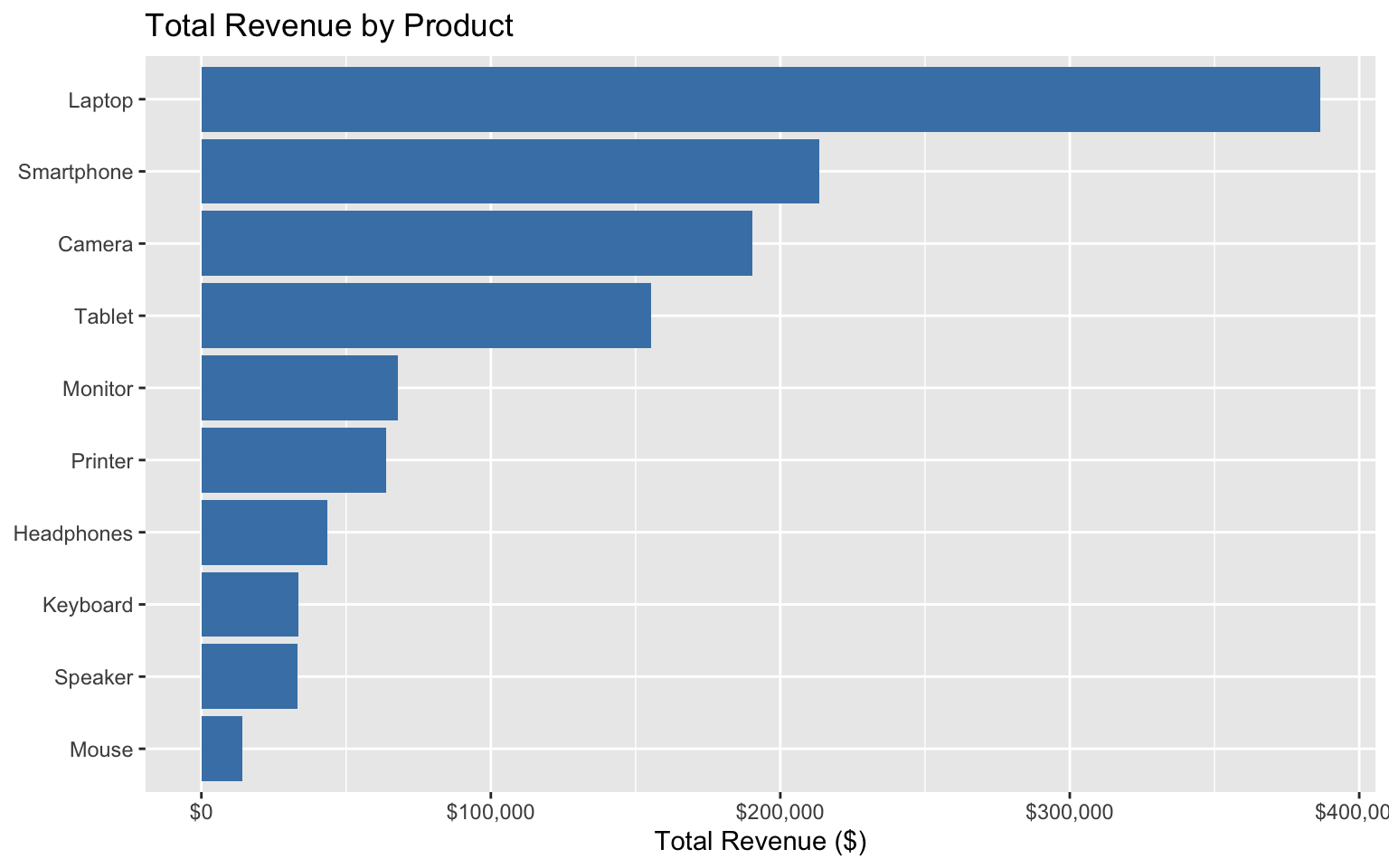

# Plot sales by month
ggplot(monthly_sales, aes(x = month, y = total_revenue, group = 1)) +
  geom_line(color = "steelblue", size = 1) +
  geom_point(color = "steelblue", size = 3) +
  labs(
    title = "Monthly Sales Trend",
    x = NULL,
    y = "Total Revenue ($)"
  ) +
  scale_y_continuous(labels = dollar_format())

Warning: Using `size` aesthetic for lines was deprecated in ggplot2 3.4.0.
ℹ Please use `linewidth` instead.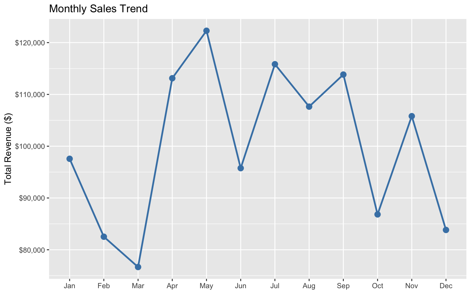

# Plot sales by category and region
ggplot(category_region_sales, aes(x = category, y = total_revenue, fill = region)) +
  geom_col(position = "dodge") +
  labs(
    title = "Sales by Category and Region",
    x = NULL,
    y = "Total Revenue ($)"
  ) +
  scale_y_continuous(labels = dollar_format()) +
  theme(axis.text.x = element_text(angle = 45, hjust = 1))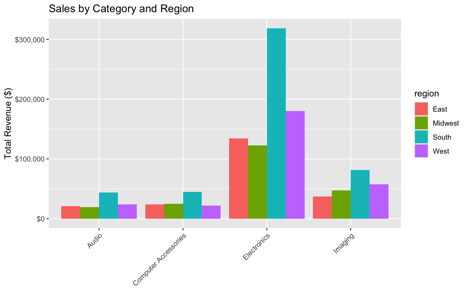

Business Insights

Based on our analysis, we can provide the following insights:

Top-Performing Products: Laptops and smartphones generate the highest revenue.
Regional Performance: The East region has the highest sales, followed by the West.
Seasonal Trends: Sales peak during certain months, suggesting seasonal patterns.
Category Performance: Electronics is the best-performing category across all regions.

Recommendations

Inventory Management: Ensure adequate stock of high-revenue products, especially during peak months.
Regional Focus: Investigate why certain regions perform better and apply successful strategies to underperforming regions.
Product Mix: Consider expanding the range of high-performing product categories.
Seasonal Promotions: Plan promotions around seasonal trends to maximize sales.

1.12 Exercises

Exercise 1: Data Import and Exploration

Import the built-in diamonds dataset from the ggplot2 package.
Explore the dataset using functions like glimpse(), summary(), and skim().
How many observations and variables are in the dataset?
What are the different categories of the cut variable?
What is the average price of diamonds in the dataset?

Exercise 2: Data Transformation

Using the diamonds dataset:

Filter the dataset to include only diamonds with a cut of “Premium” or “Ideal”.
Create a new variable called price_per_carat that calculates the price divided by carat.
Find the average price_per_carat for each color category.
Arrange the results in descending order of average price_per_carat.

Exercise 3: Data Joining

Create two datasets: one with customer information (customer ID, name, email) and one with order information (order ID, customer ID, product, amount).
Join the datasets to create a complete view of orders with customer information.
Find the total amount spent by each customer.
Identify customers who haven’t placed any orders.

Exercise 4: Business Application

You’re given a dataset of employee information including department, salary, hire date, and performance ratings:

Calculate the average salary by department.
Identify departments with above-average employee performance.
Analyze how salary relates to performance and tenure.
Create a visualization showing the relationship between tenure and salary for different departments.

1.13 Summary

In this chapter, we’ve covered the computational foundations for strategic business analytics using R and the Tidyverse ecosystem. We’ve learned how to:

Set up and navigate the R and RStudio environment
Import and export data in various formats
Transform and manipulate data using dplyr
Create and modify variables
Filter, arrange, and summarize data
Perform group-wise operations
Join multiple datasets
Handle missing data and outliers
Apply functions to data using iteration

These foundational skills will serve as the building blocks for more advanced analytics techniques in the following chapters. By mastering these skills, you’ll be well-equipped to tackle a wide range of business analytics challenges.

1.14 References

Wickham, H., & Grolemund, G. (2017). R for Data Science: Import, Tidy, Transform, Visualize, and Model Data. O’Reilly Media. https://r4ds.hadley.nz/
Wickham, H., et al. (2019). Welcome to the Tidyverse. Journal of Open Source Software, 4(43), 1686. https://doi.org/10.21105/joss.01686
Wickham, H. (2016). ggplot2: Elegant Graphics for Data Analysis. Springer. https://ggplot2-book.org/