# Install required packages if not already installed
if (!require("tidyverse")) install.packages("tidyverse")
if (!require("fixest")) install.packages("fixest")
if (!require("modelsummary")) install.packages("modelsummary")
if (!require("performance")) install.packages("performance")
if (!require("car")) install.packages("car")
if (!require("lmtest")) install.packages("lmtest")
if (!require("sandwich")) install.packages("sandwich")
if (!require("ggeffects")) install.packages("ggeffects")
if (!require("marginaleffects")) install.packages("marginaleffects")
if (!require("broom")) install.packages("broom")3 📈 Predictive Modeling I: Regression Analysis & Model Diagnostics
3.1 Learning Objectives
By the end of this chapter, you will be able to:
- Understand the principles of regression analysis for business applications
- Implement multiple linear regression models in R
- Apply non-linear regression techniques
- Use the feols package for efficient fixed effects regression
- Understand and implement fixed effects models to control for unobserved heterogeneity
- Identify and address multicollinearity using VIF analysis
- Interpret regression results in business contexts
- Perform model diagnostics to validate regression assumptions
- Compare and select models based on statistical criteria
- Visualize regression results for business presentations
3.2 Prerequisites
For this chapter, you’ll need:
- R and RStudio installed on your computer
- Understanding of data manipulation with dplyr (covered in Chapter 1)
- Basic knowledge of data visualization with ggplot2 (covered in Chapter 2)
- The following R packages installed:
# Load required packages
library(tidyverse)       # For data manipulation and visualization
library(fixest)          # For fixed effects regression
library(modelsummary)    # For creating tables of model results
library(performance)     # For model diagnostics
library(car)             # For additional regression diagnostics
library(lmtest)          # For hypothesis tests
library(sandwich)        # For robust standard errors
library(ggeffects)       # For visualizing effects
library(marginaleffects) # For calculating marginal effects
library(broom)           # For tidying model output
3.3 Introduction to Regression Analysis
Regression analysis is a statistical method for estimating the relations between a dependent variable and one or more independent variables. It’s one of the most widely used techniques in business analytics for prediction and understanding relations in data.
Why Regression Analysis in Business?
Regression analysis is valuable in business for several reasons:
- Prediction: Forecasting sales, demand, customer behavior, and other business metrics
- Understanding Relations: Identifying factors that influence business outcomes
- Quantifying Effects: Measuring the impact of different variables on business performance
- Decision Making: Informing strategic decisions based on data-driven insights
- Optimization: Finding the optimal levels of controllable factors to maximize outcomes
Types of Regression Models
There are several types of regression models, each suited for different types of data and relations:
- Simple Linear Regression: One dependent variable and one independent variable
- Multiple Linear Regression: One dependent variable and multiple independent variables
- Polynomial Regression: For modeling non-linear relations
- Fixed Effects Regression: For panel data with time-invariant effects
- Logistic Regression: For binary dependent variables (covered in Chapter 4)
- Other Non-linear Models: For various non-linear relations
3.4 Simple Linear Regression
Simple linear regression models the relation between two variables using a straight line.
The Simple Linear Regression Model
The simple linear regression model is:
\[Y = \beta_0 + \beta_1 X + \varepsilon\]
Where: - \(Y\) is the dependent variable - \(X\) is the independent variable - \(\beta_0\) is the intercept - \(\beta_1\) is the slope - \(\varepsilon\) is the error term
Implementing Simple Linear Regression in R
Let’s start with a simple example using the built-in mtcars dataset:
# Load the mtcars dataset
data(mtcars)

# Explore the data
glimpse(mtcars)
Rows: 32
Columns: 11
$ mpg <dbl> 21.0, 21.0, 22.8, 21.4, 18.7, 18.1, 14.3, 24.4, 22.8, 19.2, 17.8,…
$ cyl <dbl> 6, 6, 4, 6, 8, 6, 8, 4, 4, 6, 6, 8, 8, 8, 8, 8, 8, 4, 4, 4, 4, 8,…
$ disp <dbl> 160.0, 160.0, 108.0, 258.0, 360.0, 225.0, 360.0, 146.7, 140.8, 16…
$ hp <dbl> 110, 110, 93, 110, 175, 105, 245, 62, 95, 123, 123, 180, 180, 180…
$ drat <dbl> 3.90, 3.90, 3.85, 3.08, 3.15, 2.76, 3.21, 3.69, 3.92, 3.92, 3.92,…
$ wt <dbl> 2.620, 2.875, 2.320, 3.215, 3.440, 3.460, 3.570, 3.190, 3.150, 3.…
$ qsec <dbl> 16.46, 17.02, 18.61, 19.44, 17.02, 20.22, 15.84, 20.00, 22.90, 18…
$ vs <dbl> 0, 0, 1, 1, 0, 1, 0, 1, 1, 1, 1, 0, 0, 0, 0, 0, 0, 1, 1, 1, 1, 0,…
$ am <dbl> 1, 1, 1, 0, 0, 0, 0, 0, 0, 0, 0, 0, 0, 0, 0, 0, 0, 1, 1, 1, 0, 0,…
$ gear <dbl> 4, 4, 4, 3, 3, 3, 3, 4, 4, 4, 4, 3, 3, 3, 3, 3, 3, 4, 4, 4, 3, 3,…
$ carb <dbl> 4, 4, 1, 1, 2, 1, 4, 2, 2, 4, 4, 3, 3, 3, 4, 4, 4, 1, 2, 1, 1, 2,…# Create a scatter plot
ggplot(mtcars, aes(x = wt, y = mpg)) +
geom_point() +
geom_smooth(method = "lm", se = TRUE) +
labs(
title = "Relation between Weight and Fuel Efficiency",
x = "Weight (1000 lbs)",
y = "Miles per Gallon"
) +
theme_minimal()`geom_smooth()` using formula = 'y ~ x'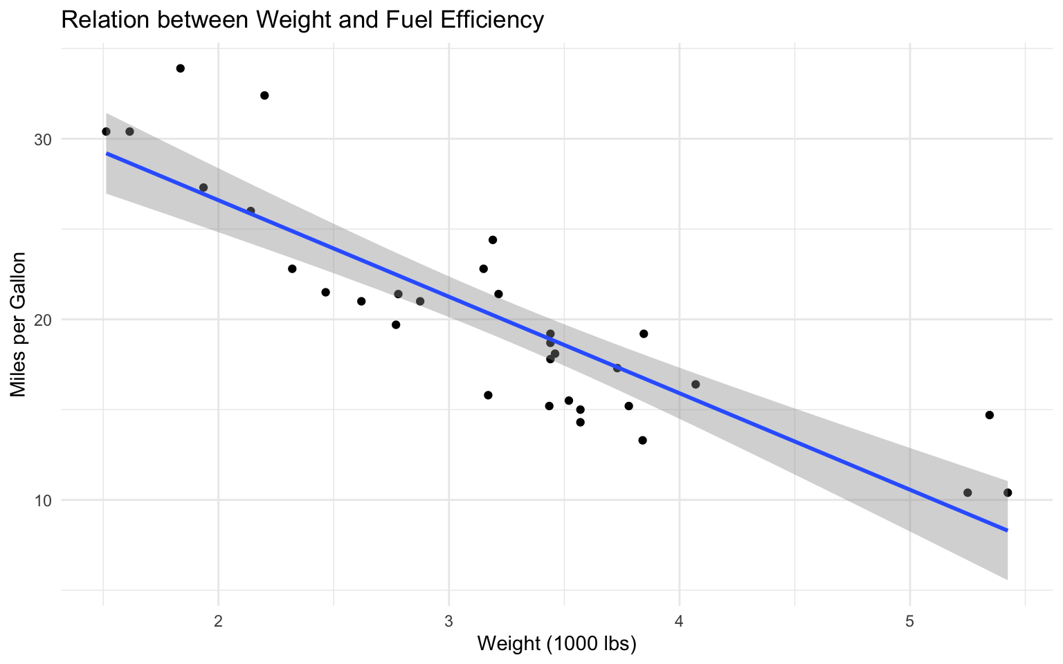
# Fit a simple linear regression model
model1 <- lm(mpg ~ wt, data = mtcars)

# View the model summary
summary(model1)
Call:
lm(formula = mpg ~ wt, data = mtcars)

Residuals:
    Min      1Q  Median      3Q     Max
-4.5432 -2.3647 -0.1252  1.4096  6.8727

Coefficients:
            Estimate Std. Error t value Pr(>|t|)
(Intercept)  37.2851     1.8776  19.858  < 2e-16 ***
wt           -5.3445     0.5591  -9.559 1.29e-10 ***
---
Signif. codes:  0 '***' 0.001 '**' 0.01 '*' 0.05 '.' 0.1 ' ' 1

Residual standard error: 3.046 on 30 degrees of freedom
Multiple R-squared:  0.7528,    Adjusted R-squared:  0.7446
F-statistic: 91.38 on 1 and 30 DF,  p-value: 1.294e-10
Interpreting the Results
The model output provides several important pieces of information:
- Coefficients: The estimated values of \(\beta_0\) and \(\beta_1\)
- Standard Errors: The uncertainty in the coefficient estimates
- t-values and p-values: Tests of statistical significance
- R-squared: The proportion of variance explained by the model
- F-statistic: Test of overall model significance
In our example: - The intercept (\(\beta_0\)) is 37.2851262, meaning a car with zero weight would have an estimated MPG of 37.2851262 (not meaningful in this context). - The slope (\(\beta_1\)) is -5.3444716, meaning for each additional 1,000 lbs of weight, MPG decreases by 5.3444716 on average. - The R-squared is 0.7528328, indicating that 75.3% of the variation in MPG is explained by weight.
Making Predictions
We can use the model to make predictions:
# Create new data for prediction
new_cars <- data.frame(wt = c(2.5, 3.0, 3.5))

# Make predictions
predictions <- predict(model1, newdata = new_cars, interval = "confidence")

# View the predictions
cbind(new_cars, predictions)
wt fit lwr upr
1 2.5 23.92395 22.55284 25.29506
2 3.0 21.25171 20.12444 22.37899
3 3.5 18.57948 17.43342 19.725533.5 Multiple Linear Regression
Multiple linear regression extends simple linear regression to include multiple independent variables.
The Multiple Linear Regression Model
The multiple linear regression model is:
\[Y = \beta_0 + \beta_1 X_1 + \beta_2 X_2 + \ldots + \beta_p X_p + \varepsilon\]
Where: - \(Y\) is the dependent variable - \(X_1, X_2, \ldots, X_p\) are the independent variables - \(\beta_0, \beta_1, \beta_2, \ldots, \beta_p\) are the coefficients - \(\varepsilon\) is the error term
Implementing Multiple Linear Regression in R
Let’s extend our example to include multiple predictors:
# Fit a multiple linear regression model
model2 <- lm(mpg ~ wt + hp + disp, data = mtcars)

# View the model summary
summary(model2)
Call:
lm(formula = mpg ~ wt + hp + disp, data = mtcars)

Residuals:
   Min     1Q Median     3Q    Max
-3.891 -1.640 -0.172  1.061  5.861

Coefficients:
             Estimate Std. Error t value Pr(>|t|)
(Intercept) 37.105505   2.110815  17.579  < 2e-16 ***
wt          -3.800891   1.066191  -3.565  0.00133 **
hp          -0.031157   0.011436  -2.724  0.01097 *
disp        -0.000937   0.010350  -0.091  0.92851
---
Signif. codes:  0 '***' 0.001 '**' 0.01 '*' 0.05 '.' 0.1 ' ' 1

Residual standard error: 2.639 on 28 degrees of freedom
Multiple R-squared:  0.8268,    Adjusted R-squared:  0.8083
F-statistic: 44.57 on 3 and 28 DF,  p-value: 8.65e-11
Interpreting Multiple Regression Results
In multiple regression, each coefficient represents the effect of the corresponding variable, holding all other variables constant. This is known as the “ceteris paribus” interpretation.
In our example: - The coefficient for wt is -3.8008906, meaning for each additional 1,000 lbs of weight, MPG decreases by 3.8008906 on average, holding horsepower and displacement constant. - The coefficient for hp is -0.0311566, meaning for each additional horsepower, MPG decreases by 0.0311566 on average, holding weight and displacement constant. - The R-squared is 0.8268361, indicating that 82.7% of the variation in MPG is explained by the model.
Comparing Models
We can compare models using various criteria:
# Compare models using modelsummary
modelsummary(
  list(
    "Model 1" = model1,
    "Model 2" = model2
  ),
  stars = TRUE,
  gof_map = c("nobs", "r.squared", "adj.r.squared", "AIC", "BIC")
)| Model 1 | Model 2 | |
|---|---|---|
| + p < 0.1, * p < 0.05, ** p < 0.01, *** p < 0.001 | ||
| (Intercept) | 37.285*** | 37.106*** |
| (1.878) | (2.111) | |
| wt | -5.344*** | -3.801** |
| (0.559) | (1.066) | |
| hp | -0.031* | |
| (0.011) | ||
| disp | -0.001 | |
| (0.010) | ||
| Num.Obs. | 32 | 32 |
| R2 | 0.753 | 0.827 |
| R2 Adj. | 0.745 | 0.808 |
We can also use the anova() function to formally test whether adding variables improves the model:
# Compare nested models
anova(model1, model2)
Analysis of Variance Table
Model 1: mpg ~ wt
Model 2: mpg ~ wt + hp + disp
Res.Df RSS Df Sum of Sq F Pr(>F)
1 30 278.32
2 28 194.99 2 83.331 5.983 0.006863 **
---
Signif. codes: 0 '***' 0.001 '**' 0.01 '*' 0.05 '.' 0.1 ' ' 1A significant p-value indicates that the more complex model (model2) provides a significantly better fit than the simpler model (model1).
3.6 Model Diagnostics
Regression models rely on several assumptions. We need to check these assumptions to ensure the validity of our results.
Key Regression Assumptions
- Linearity: The relation between the dependent and independent variables is linear.
- Independence: The observations are independent of each other.
- Homoscedasticity: The variance of the residuals is constant across all levels of the independent variables.
- Normality: The residuals are normally distributed.
- No Multicollinearity: The independent variables are not highly correlated with each other.
- No Influential Outliers: There are no extreme values that disproportionately influence the results.
Checking Assumptions with Diagnostic Plots
R provides several diagnostic plots for checking regression assumptions:
# Basic diagnostic plots
par(mfrow = c(2, 2))
plot(model2)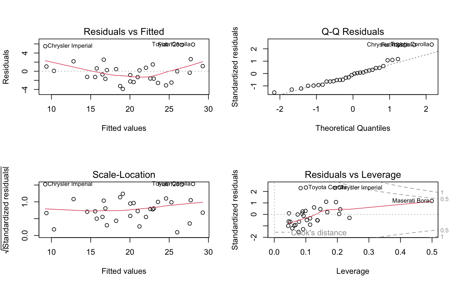
par(mfrow = c(1, 1))These plots help us check: 1. Residuals vs Fitted: Checks linearity and homoscedasticity 2. Normal Q-Q: Checks normality of residuals 3. Scale-Location: Another check for homoscedasticity 4. Residuals vs Leverage: Identifies influential observations
Advanced Diagnostics
We can use the performance package for more comprehensive diagnostics:
# Check model assumptions
check_model(model2)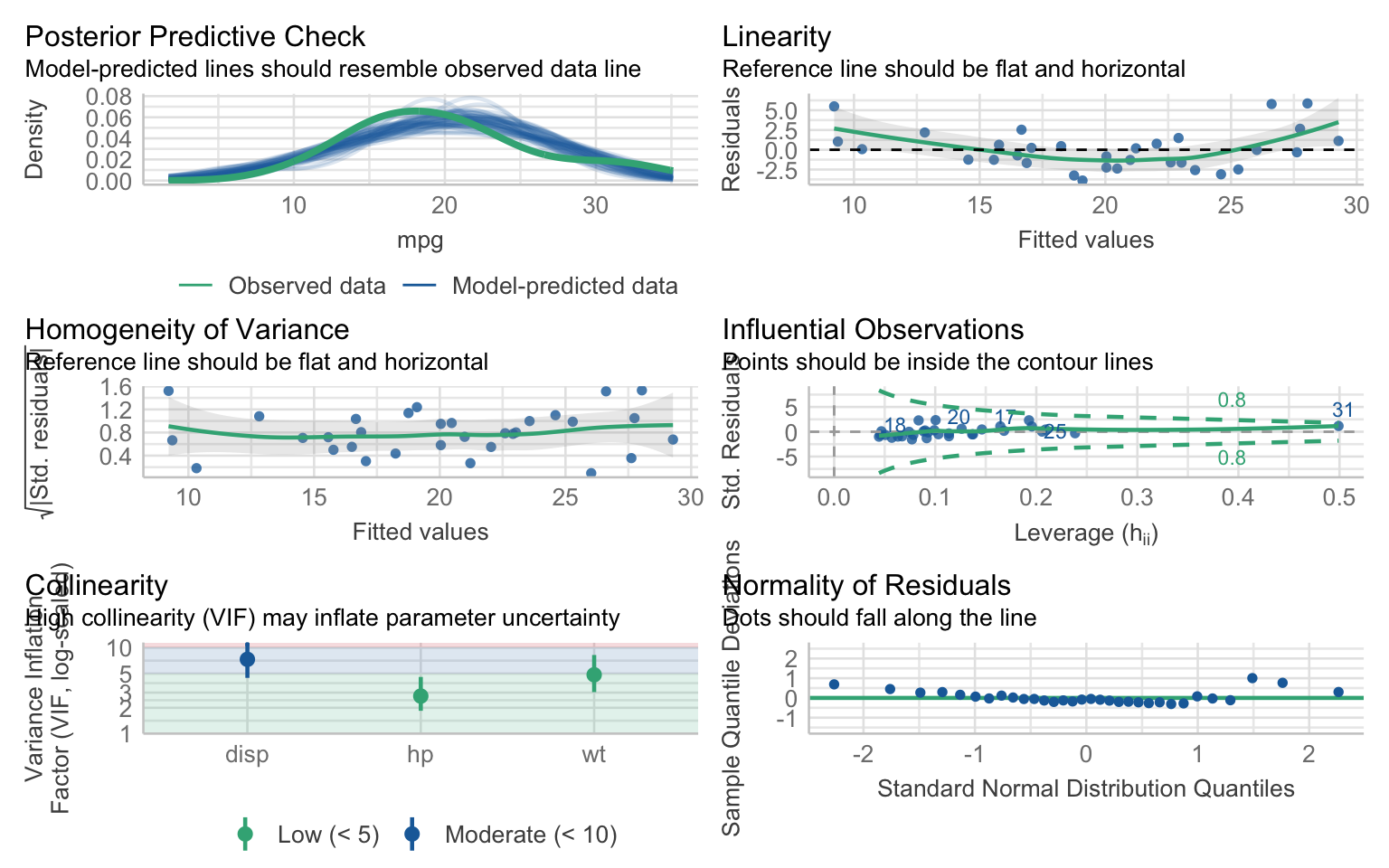
3.7 Multicollinearity and VIF Analysis
Multicollinearity is a critical issue in regression analysis that occurs when independent variables are highly correlated with each other. This section explores how to detect, understand, and address multicollinearity in your regression models.
Understanding Multicollinearity
Multicollinearity occurs when two or more independent variables in a regression model are highly correlated. This creates several problems:
- Unstable Coefficient Estimates: Small changes in the data can lead to large changes in the estimated coefficients.
- Inflated Standard Errors: The standard errors of the coefficients become larger, making it harder to detect significant relations.
- Reduced Statistical Power: The model’s ability to identify significant relations is diminished.
- Difficult Interpretation: It becomes challenging to isolate the effect of individual variables.
Detecting Multicollinearity
Correlation Matrix
A simple first step is to examine the correlation matrix of your independent variables:
# Create correlation matrix for independent variables in the mtcars dataset
cor_matrix <- cor(mtcars[, c("wt", "hp", "disp", "cyl", "drat")])
round(cor_matrix, 3)
wt hp disp cyl drat
wt 1.000 0.659 0.888 0.782 -0.712
hp 0.659 1.000 0.791 0.832 -0.449
disp 0.888 0.791 1.000 0.902 -0.710
cyl 0.782 0.832 0.902 1.000 -0.700
drat -0.712 -0.449 -0.710 -0.700 1.000# Visualize the correlation matrix
corrplot::corrplot(cor_matrix, method = "circle", type = "upper",
tl.col = "black", tl.srt = 45)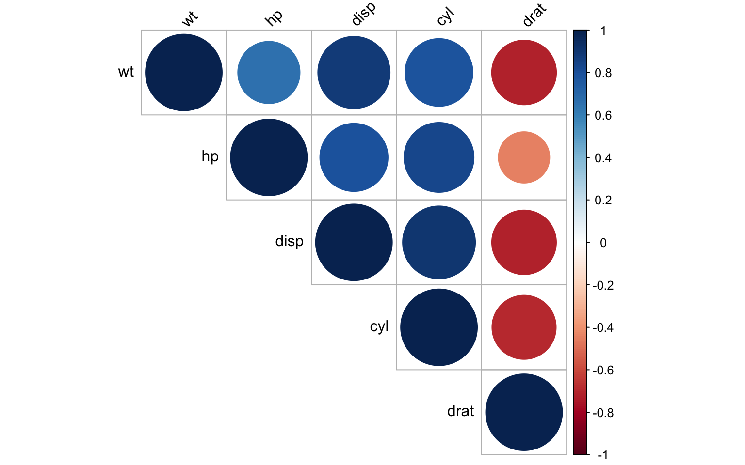
Correlation coefficients close to 1 or -1 indicate potential multicollinearity. However, correlation matrices only detect pairwise relations and may miss more complex multicollinearity involving multiple variables.
Variance Inflation Factor (VIF)
The Variance Inflation Factor (VIF) is a more comprehensive measure of multicollinearity. For each independent variable, VIF measures how much the variance of the estimated regression coefficient is increased due to multicollinearity.
The VIF for a variable \(X_j\) is calculated as:
\[VIF_j = \frac{1}{1 - R_j^2}\]
Where \(R_j^2\) is the R-squared value obtained by regressing \(X_j\) on all other independent variables.
# Create a more complex model with potential multicollinearity
model_multi <- lm(mpg ~ wt + hp + disp + cyl + drat, data = mtcars)

# Calculate VIF values
vif_values <- car::vif(model_multi)
vif_values
wt hp disp cyl drat
5.168795 3.990380 10.463957 7.869010 2.662298 Interpreting VIF Values
VIF values are interpreted as follows:
- VIF = 1: No multicollinearity
- 1 < VIF < 5: Moderate multicollinearity
- 5 < VIF < 10: High multicollinearity
- VIF > 10: Severe multicollinearity that requires attention
In our example, we can see that disp and cyl have high VIF values, indicating substantial multicollinearity with other predictors.
Addressing Multicollinearity
When multicollinearity is detected, several approaches can be taken:
2. Combine Variables
Another approach is to combine correlated variables into a single index or factor:
# Example: Create a composite "engine size" variable
mtcars$engine_size <- scale(mtcars$disp) + scale(mtcars$cyl)

# Model with the composite variable
model_composite <- lm(mpg ~ wt + hp + engine_size + drat, data = mtcars)

# Check VIF values
car::vif(model_composite)
wt hp engine_size drat
4.065587 3.909665 9.184216 2.604446 3. Use Principal Component Analysis (PCA)
PCA can transform correlated variables into a set of uncorrelated components:
# Perform PCA on the correlated variables
pca_result <- prcomp(mtcars[, c("wt", "hp", "disp", "cyl", "drat")], scale = TRUE)

# Summary of PCA
summary(pca_result)
Importance of components:
PC1 PC2 PC3 PC4 PC5
Standard deviation 1.9977 0.7593 0.50407 0.33746 0.25439
Proportion of Variance 0.7982 0.1153 0.05082 0.02278 0.01294
Cumulative Proportion 0.7982 0.9135 0.96428 0.98706 1.00000# Create a dataset with principal components
pc_data <- as.data.frame(pca_result$x[, 1:2]) # Using first two components
pc_data$mpg <- mtcars$mpg
# Fit a model using principal components
model_pca <- lm(mpg ~ PC1 + PC2, data = pc_data)
summary(model_pca)
Call:
lm(formula = mpg ~ PC1 + PC2, data = pc_data)

Residuals:
    Min      1Q  Median      3Q     Max
-3.8280 -1.6324 -0.5814  1.1879  6.1691

Coefficients:
            Estimate Std. Error t value Pr(>|t|)
(Intercept)  20.0906     0.4699  42.755  < 2e-16 ***
PC1          -2.7265     0.2390 -11.408 3.06e-12 ***
PC2           0.2877     0.6288   0.458    0.651
---
Signif. codes:  0 '***' 0.001 '**' 0.01 '*' 0.05 '.' 0.1 ' ' 1

Residual standard error: 2.658 on 29 degrees of freedom
Multiple R-squared:  0.818, Adjusted R-squared:  0.8055
F-statistic: 65.18 on 2 and 29 DF,  p-value: 1.863e-11
4. Ridge Regression
Ridge regression is a regularization technique that can handle multicollinearity by adding a penalty term to the regression:
# Load the glmnet package for ridge regression
if (!require("glmnet")) install.packages("glmnet")
Loading required package: glmnetLoading required package: MatrixWarning: package 'Matrix' was built under R version 4.4.1
Attaching package: 'Matrix'The following objects are masked from 'package:tidyr':
expand, pack, unpackLoaded glmnet 4.1-8library(glmnet)
# Prepare data for glmnet
x <- as.matrix(mtcars[, c("wt", "hp", "disp", "cyl", "drat")])
y <- mtcars$mpg
# Fit ridge regression with cross-validation to find optimal lambda
cv_ridge <- cv.glmnet(x, y, alpha = 0)
best_lambda <- cv_ridge$lambda.min
# Fit ridge regression with optimal lambda
ridge_model <- glmnet(x, y, alpha = 0, lambda = best_lambda)
# Display coefficients
coef(ridge_model)6 x 1 sparse Matrix of class "dgCMatrix"
s0
(Intercept) 32.0444326440
wt -2.5290823422
hp -0.0208093437
disp -0.0007426654
cyl -0.7701453676
drat 1.1599900587Practical Considerations for VIF in Business Analytics
In business applications, multicollinearity requires careful consideration:
Business Context: Sometimes, even with high VIF values, keeping certain variables may be important for business interpretation.
Prediction vs. Explanation: If your primary goal is prediction, multicollinearity is less problematic than if you’re trying to understand the impact of individual variables.
Domain Knowledge: Use industry expertise to decide which variables to keep or combine.
Continuous Monitoring: As new data becomes available, reassess multicollinearity as relations between variables may change over time.
Example: Addressing Multicollinearity in Marketing Mix Modeling
Let’s consider a marketing mix modeling scenario where advertising channels might be correlated:
# Create a simulated marketing dataset with multicollinearity
set.seed(123)
n <- 100

# Generate correlated advertising variables
tv_spend <- rnorm(n, mean = 50, sd = 10)
digital_spend <- 0.7 * tv_spend + rnorm(n, mean = 10, sd = 5)
social_spend <- 0.5 * digital_spend + rnorm(n, mean = 20, sd = 8)

# Generate sales with some noise
sales <- 10 + 0.3 * tv_spend + 0.2 * digital_spend + 0.1 * social_spend + rnorm(n, mean = 0, sd = 15)

# Create a data frame
marketing_data <- data.frame(
  tv_spend = tv_spend,
  digital_spend = digital_spend,
  social_spend = social_spend,
  sales = sales
)

# Check correlation
cor(marketing_data[, c("tv_spend", "digital_spend", "social_spend")])
tv_spend digital_spend social_spend
tv_spend 1.0000000 0.7865247 0.2540935
digital_spend 0.7865247 1.0000000 0.3946187
social_spend 0.2540935 0.3946187 1.0000000# Fit a model
marketing_model <- lm(sales ~ tv_spend + digital_spend + social_spend, data = marketing_data)
# Check VIF
car::vif(marketing_model) tv_spend digital_spend social_spend
2.648118 2.934047 1.196216 # Address multicollinearity by creating a composite digital variable
marketing_data$total_digital <- marketing_data$digital_spend + marketing_data$social_spend
# Fit a revised model
marketing_model_revised <- lm(sales ~ tv_spend + total_digital, data = marketing_data)
# Check VIF of the revised model
car::vif(marketing_model_revised) tv_spend total_digital
1.607237 1.607237 # Compare models
modelsummary(
list(
"Original Model" = marketing_model,
"Revised Model" = marketing_model_revised
),
stars = TRUE,
gof_map = c("nobs", "r.squared", "adj.r.squared", "AIC", "BIC")
)| Original Model | Revised Model | |
|---|---|---|
| + p < 0.1, * p < 0.05, ** p < 0.01, *** p < 0.001 | ||
| (Intercept) | 14.634 | 13.488 |
| (11.099) | (11.006) | |
| tv_spend | 0.120 | 0.274 |
| (0.283) | (0.220) | |
| digital_spend | 0.392 | |
| (0.347) | ||
| social_spend | -0.008 | |
| (0.210) | ||
| total_digital | 0.121 | |
| (0.150) | ||
| Num.Obs. | 100 | 100 |
| R2 | 0.061 | 0.054 |
| R2 Adj. | 0.032 | 0.034 |
In this example, we addressed multicollinearity by combining digital and social spending into a single variable, which reduced VIF values while maintaining the model’s explanatory power.
3.8 Fixed Effects Regression
Fixed effects regression is a powerful method for controlling for unobserved heterogeneity in panel data. This section provides a comprehensive overview of fixed effects models, their intuition, implementation, and advanced applications.
Understanding Fixed Effects
What are Fixed Effects?
Fixed effects regression allows us to control for unobserved variables that are constant over time (or within groups). This is particularly valuable when:
- We can’t figure out the correct causal diagram that tells us what to control for
- We can’t measure all the variables we need to control for
Fixed effects solves these problems by controlling for all variables, whether observed or not, as long as they stay constant within some larger category (like individual, firm, or country).
The Intuition Behind Fixed Effects
The key insight of fixed effects is simple but powerful: by controlling for the larger category (e.g., individual), we automatically control for everything that is constant within that category.
For example, if we’re studying the effect of rural towns getting electricity on their productivity, geography might be a confounder. However, geography doesn’t change over time for a given town. By including fixed effects for town, we effectively control for geography and all other time-invariant characteristics of each town.
How Fixed Effects Works: The Variation Within
Fixed effects focuses on variation within individuals or groups, rather than between them. Let’s understand this distinction:
- Between Variation: Differences across different individuals/groups (e.g., comparing one person’s average height to another person’s average height)
- Within Variation: Changes within the same individual/group over time (e.g., comparing a person’s height at different ages)
Fixed effects removes all between variation and focuses solely on within variation. This is how it controls for all time-invariant characteristics.
Visualizing Within and Between Variation
Let’s create a simple example to visualize this concept:
# Create a small panel dataset
set.seed(123)
person_data <- data.frame(
  person = rep(c("You", "Me"), each = 5),
  year = rep(2018:2022, 2),
  exercise = c(5, 6, 4, 7, 5,  # Your exercise hours
               3, 4, 2, 3, 4),  # My exercise hours
  colds = c(3, 2, 4, 1, 3,      # Your number of colds
            6, 5, 7, 6, 4)      # My number of colds
)

# Calculate person-specific means
person_means <- person_data %>%
  group_by(person) %>%
  summarize(
    mean_exercise = mean(exercise),
    mean_colds = mean(colds)
  )

# Add the means and calculate within-person variation
person_data <- person_data %>%
  left_join(person_means, by = "person") %>%
  mutate(
    exercise_within = exercise - mean_exercise,
    colds_within = colds - mean_colds
  )

# Plot the raw data
p1 <- ggplot(person_data, aes(x = exercise, y = colds, color = person)) +
  geom_point(size = 3) +
  geom_smooth(method = "lm", se = FALSE) +
  labs(title = "Raw Data: Exercise vs. Colds",
       x = "Exercise (hours/week)",
       y = "Number of Colds per Year") +
  theme_minimal()

# Plot the person means (between variation)
p2 <- ggplot(person_means, aes(x = mean_exercise, y = mean_colds, color = person)) +
  geom_point(size = 5) +
  geom_line() +
  labs(title = "Between Variation: Person Averages",
       x = "Average Exercise (hours/week)",
       y = "Average Number of Colds per Year") +
  theme_minimal()

# Plot the within-person variation
p3 <- ggplot(person_data, aes(x = exercise_within, y = colds_within, color = person)) +
  geom_point(size = 3) +
  geom_smooth(method = "lm", se = FALSE) +
  labs(title = "Within Variation: Deviations from Person Means",
       x = "Exercise Deviation from Personal Average",
       y = "Colds Deviation from Personal Average") +
  theme_minimal() +
  geom_hline(yintercept = 0, linetype = "dashed") +
  geom_vline(xintercept = 0, linetype = "dashed")

# Combine plots
gridExtra::grid.arrange(p1, p2, p3, ncol = 2)
`geom_smooth()` using formula = 'y ~ x'
`geom_line()`: Each group consists of only one observation.
ℹ Do you need to adjust the group aesthetic?
`geom_smooth()` using formula = 'y ~ x'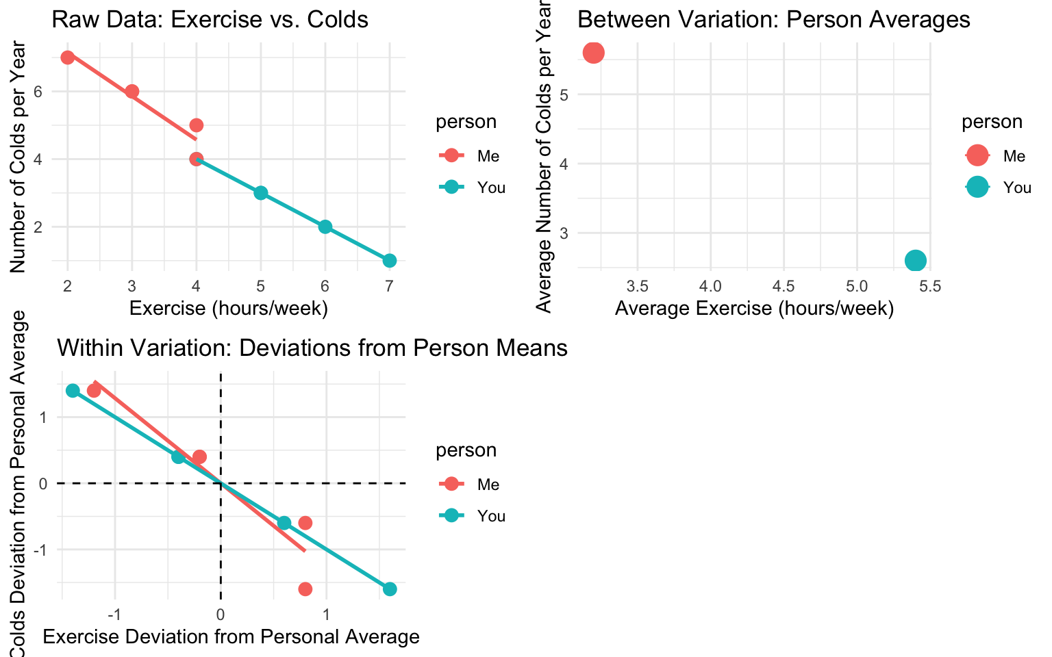
In this example: - The first plot shows the raw data with a negative relations between exercise and colds - The second plot shows the between-person variation (person averages) - The third plot shows the within-person variation (deviations from personal averages)
The relation in the within-person variation (third plot) represents what fixed effects regression would estimate.
Fixed Effects in Action
Let’s see how fixed effects works with a more realistic example:
# Create a simulated panel dataset
set.seed(123)

# Number of firms and time periods
n_firms <- 50
n_years <- 10

# Create panel data
panel_data <- expand.grid(
  firm_id = 1:n_firms,
  year = 2010:(2010 + n_years - 1)
) %>%
  as_tibble() %>%
  # Add firm fixed effect (time-invariant)
  group_by(firm_id) %>%
  mutate(
    firm_size = rnorm(1, mean = 5, sd = 2),
    firm_quality = rnorm(1, mean = 0, sd = 1)
  ) %>%
  # Add time fixed effect
  group_by(year) %>%
  mutate(
    market_condition = rnorm(1, mean = 0, sd = 0.5)
  ) %>%
  # Add time-varying variables
  ungroup() %>%
  mutate(
    investment = 0.1 * firm_size + 0.05 * (year - 2010) + 0.2 * market_condition + rnorm(n(), mean = 0, sd = 0.5),
    advertising = 0.2 * firm_size + 0.1 * firm_quality + rnorm(n(), mean = 0, sd = 0.3),
    # Outcome variable
    revenue = 2 * firm_size + 0.5 * firm_quality + 1.5 * investment + 0.8 * advertising +
              0.3 * market_condition + rnorm(n(), mean = 0, sd = 1)
  )

# View the data structure
glimpse(panel_data)
Rows: 500
Columns: 8
$ firm_id <int> 1, 2, 3, 4, 5, 6, 7, 8, 9, 10, 11, 12, 13, 14, 15, 16…
$ year <int> 2010, 2010, 2010, 2010, 2010, 2010, 2010, 2010, 2010,…
$ firm_size <dbl> 3.879049, 4.539645, 8.117417, 5.141017, 5.258575, 8.4…
$ firm_quality <dbl> 0.25331851, -0.02854676, -0.04287046, 1.36860228, -0.…
$ market_condition <dbl> -0.3552033, -0.3552033, -0.3552033, -0.3552033, -0.35…
$ investment <dbl> 0.02919073, 0.68690601, -0.06824035, 0.41528004, 0.71…
$ advertising <dbl> 0.6820324, 0.5397943, 2.1254731, 1.1602628, 1.3516215…
$ revenue <dbl> 7.742679, 11.377814, 20.129344, 11.494925, 13.508447,…Implementing Fixed Effects Regression
There are several ways to implement fixed effects regression:
1. Using Binary Indicators
One approach is to include binary indicators for each individual/group:
# Fit a model with binary indicators for firm_id
# Note: This is computationally intensive with many firms
model_dummies <- lm(revenue ~ investment + advertising + factor(firm_id), data = panel_data)

# Display partial results
summary(model_dummies)$coefficients[1:5, ]
Estimate Std. Error t value Pr(>|t|)
(Intercept) 8.0289278 0.34680651 23.151029 1.463859e-78
investment 1.6637704 0.08839923 18.821096 1.189134e-58
advertising 0.7270425 0.14714269 4.941071 1.099369e-06
factor(firm_id)2 1.0617453 0.43123398 2.462110 1.418777e-02
factor(firm_id)3 8.5384539 0.44253602 19.294371 8.055158e-612. Demeaning (Within Transformation)
A more efficient approach is to subtract the individual/group means:
# Calculate firm means
firm_means <- panel_data %>%
  group_by(firm_id) %>%
  summarize(
    mean_revenue = mean(revenue),
    mean_investment = mean(investment),
    mean_advertising = mean(advertising)
  )

# Merge means and calculate within variation
panel_data_within <- panel_data %>%
  left_join(firm_means, by = "firm_id") %>%
  mutate(
    revenue_within = revenue - mean_revenue,
    investment_within = investment - mean_investment,
    advertising_within = advertising - mean_advertising
  )

# Fit model using within variation
model_within <- lm(revenue_within ~ investment_within + advertising_within - 1, data = panel_data_within)
summary(model_within)
Call:
lm(formula = revenue_within ~ investment_within + advertising_within -
    1, data = panel_data_within)

Residuals:
    Min      1Q  Median      3Q     Max
-2.6679 -0.5634  0.0397  0.6343  3.2572

Coefficients:
                   Estimate Std. Error t value Pr(>|t|)
investment_within   1.66377    0.08384   19.84  < 2e-16 ***
advertising_within  0.72704    0.13956    5.21 2.78e-07 ***
---
Signif. codes:  0 '***' 0.001 '**' 0.01 '*' 0.05 '.' 0.1 ' ' 1

Residual standard error: 0.9143 on 498 degrees of freedom
Multiple R-squared:  0.4554,    Adjusted R-squared:  0.4533
F-statistic: 208.3 on 2 and 498 DF,  p-value: < 2.2e-16
3. Using the fixest Package
The most efficient and user-friendly approach is to use the fixest package:
# Pooled OLS (no fixed effects)
model_pooled <- feols(revenue ~ investment + advertising, data = panel_data)

# Firm fixed effects
model_firm_fe <- feols(revenue ~ investment + advertising | firm_id, data = panel_data)

# Compare models
etable(model_pooled, model_firm_fe)
model_pooled model_firm_fe
Dependent Var.: revenue revenue
Constant 3.583*** (0.2716)
investment 2.842*** (0.2072) 1.664*** (0.0949)
advertising 6.250*** (0.2332) 0.7270*** (0.1428)
Fixed-Effects: ----------------- ------------------
firm_id No Yes
_______________ _________________ __________________
S.E. type IID by: firm_id
Observations 500 500
R2 0.70199 0.95911
Within R2 -- 0.45544
---
Signif. codes: 0 '***' 0.001 '**' 0.01 '*' 0.05 '.' 0.1 ' ' 1Interpreting Fixed Effects Results
The interpretation of coefficients in fixed effects models is similar to regular regression, but with an important distinction:
- Coefficients represent the effect of a one-unit change in the independent variable on the dependent variable, within the same individual/group.
For example, in our firm fixed effects model, the coefficient for investment (1.49) means that for a given firm, a one-unit increase in investment is associated with a 1.49-unit increase in revenue, on average.
The fixed effects themselves (not shown in the output) represent the time-invariant characteristics of each firm.
Multiple Sets of Fixed Effects
We can include multiple sets of fixed effects to control for different sources of unobserved heterogeneity:
Two-way Fixed Effects
Two-way fixed effects include fixed effects for both individuals/groups and time periods:
# Two-way fixed effects (firm and year)
model_twoway_fe <- feols(revenue ~ investment + advertising | firm_id + year, data = panel_data)

# Compare models
etable(model_firm_fe, model_twoway_fe)
model_firm_fe model_twoway_fe
Dependent Var.: revenue revenue
investment 1.664*** (0.0949) 1.639*** (0.0958)
advertising 0.7270*** (0.1428) 0.7241*** (0.1493)
Fixed-Effects: ------------------ ------------------
firm_id Yes Yes
year No Yes
_______________ __________________ __________________
S.E.: Clustered by: firm_id by: firm_id
Observations 500 500
R2 0.95911 0.95959
Within R2 0.45544 0.42077
---
Signif. codes: 0 '***' 0.001 '**' 0.01 '*' 0.05 '.' 0.1 ' ' 1In the two-way fixed effects model, we control for both: 1. Time-invariant characteristics of each firm (firm fixed effects) 2. Firm-invariant characteristics of each year (year fixed effects)
This is particularly useful when there are both individual-specific and time-specific unobserved factors that might confound the relation of interest.
Advanced Topics in Fixed Effects
Clustered Standard Errors
When using fixed effects, it’s often recommended to use clustered standard errors to account for potential correlation in the error terms within groups:
# Fixed effects with clustered standard errors
model_fe_clustered <- feols(revenue ~ investment + advertising | firm_id,
                           cluster = "firm_id",
                           data = panel_data)

# Compare with and without clustering
etable(model_firm_fe, model_fe_clustered)
model_firm_fe model_fe_clustered
Dependent Var.: revenue revenue
investment 1.664*** (0.0949) 1.664*** (0.0949)
advertising 0.7270*** (0.1428) 0.7270*** (0.1428)
Fixed-Effects: ------------------ ------------------
firm_id Yes Yes
_______________ __________________ __________________
S.E.: Clustered by: firm_id by: firm_id
Observations 500 500
R2 0.95911 0.95911
Within R2 0.45544 0.45544
---
Signif. codes: 0 '***' 0.001 '**' 0.01 '*' 0.05 '.' 0.1 ' ' 1Fixed Effects vs. Random Effects
While fixed effects removes all between variation, random effects uses a weighted average of within and between variation:
# Random effects model
if (!require("plm")) install.packages("plm")
Loading required package: plmRegistered S3 method overwritten by 'lfe':
method from
nobs.felm broom
Attaching package: 'plm'The following objects are masked from 'package:dplyr':
between, lag, leadlibrary(plm)
# Convert to panel data format
panel_data_plm <- pdata.frame(panel_data, index = c("firm_id", "year"))
# Fit random effects model
model_re <- plm(revenue ~ investment + advertising,
data = panel_data_plm,
model = "random")
# Compare fixed effects and random effects
summary(model_re)Oneway (individual) effect Random Effect Model
(Swamy-Arora's transformation)
Call:
plm(formula = revenue ~ investment + advertising, data = panel_data_plm,
model = "random")
Balanced Panel: n = 50, T = 10, N = 500
Effects:
var std.dev share
idiosyncratic 0.9292 0.9640 0.538
individual 0.7977 0.8931 0.462
theta: 0.677
Residuals:
Min. 1st Qu. Median 3rd Qu. Max.
-4.224431 -0.834830 -0.022734 0.840686 4.498583
Coefficients:
Estimate Std. Error z-value Pr(>|z|)
(Intercept) 8.45068 0.30038 28.134 < 2.2e-16 ***
investment 1.95363 0.12981 15.050 < 2.2e-16 ***
advertising 2.15531 0.20114 10.716 < 2.2e-16 ***
---
Signif. codes: 0 '***' 0.001 '**' 0.01 '*' 0.05 '.' 0.1 ' ' 1
Total Sum of Squares: 1747
Residual Sum of Squares: 1024.5
R-Squared: 0.41355
Adj. R-Squared: 0.41119
Chisq: 350.476 on 2 DF, p-value: < 2.22e-16The key difference is that random effects assumes the individual effects are uncorrelated with the independent variables, while fixed effects does not make this assumption.
Hausman Test
The Hausman test can help decide between fixed effects and random effects:
# Fit fixed effects model using plm
model_fe_plm <- plm(revenue ~ investment + advertising,
                   data = panel_data_plm,
                   model = "within")

# Perform Hausman test
phtest(model_fe_plm, model_re)
    Hausman Test

data:  revenue ~ investment + advertising
chisq = 123.43, df = 2, p-value < 2.2e-16
alternative hypothesis: one model is inconsistent
A significant p-value suggests that fixed effects is more appropriate than random effects.
Fixed Effects in Non-linear Models
Fixed effects can also be applied to non-linear models, though the implementation is more complex:
# Create a binary outcome
panel_data$high_revenue <- ifelse(panel_data$revenue > median(panel_data$revenue), 1, 0)

# Logit model with fixed effects using fixest package
# We already loaded fixest at the beginning of the document

# Fit logit model with firm fixed effects
logit_fe <- feglm(high_revenue ~ investment + advertising | firm_id,
                 family = binomial,
                 data = panel_data)
NOTE: 31 fixed-effects (310 observations) removed because of only 0 (or only 1) outcomes.summary(logit_fe)GLM estimation, family = binomial, Dep. Var.: high_revenue
Observations: 190
Fixed-effects: firm_id: 19
Standard-errors: Clustered (firm_id)
Estimate Std. Error z value Pr(>|z|)
investment 3.11163 0.806970 3.85594 0.00011528 ***
advertising 2.04345 0.811017 2.51962 0.01174811 *
---
Signif. codes: 0 '***' 0.001 '**' 0.01 '*' 0.05 '.' 0.1 ' ' 1
Log-Likelihood: -72.9 Adj. Pseudo R2: 0.29284
BIC: 256.1 Squared Cor.: 0.532328Business Applications of Fixed Effects
Fixed effects regression has numerous applications in business analytics:
Marketing: Controlling for individual customer characteristics when analyzing the effect of marketing campaigns on purchase behavior
Finance: Controlling for firm-specific factors when studying the impact of policy changes on stock returns
HR Analytics: Controlling for employee characteristics when analyzing the effect of training programs on productivity
Operations: Controlling for store-specific factors when evaluating the impact of process changes on efficiency
Economics: Controlling for country-specific factors when studying the effect of policy changes on economic outcomes
Example: Store Performance Analysis
Let’s apply fixed effects to a business case of store performance analysis:
# Create a simulated store performance dataset
set.seed(456)
n_stores <- 50
n_months <- 24

# Create store performance data
store_data <- expand.grid(
  store_id = 1:n_stores,
  month = 1:n_months
) %>%
  as_tibble() %>%
  # Add store fixed effects (time-invariant)
  group_by(store_id) %>%
  mutate(
    store_size = rnorm(1, mean = 10000, sd = 3000),
    location_quality = rnorm(1, mean = 0, sd = 1),
    manager_skill = rnorm(1, mean = 0, sd = 1)
  ) %>%
  # Add time fixed effects
  group_by(month) %>%
  mutate(
    seasonality = sin(month * pi/6) * 2,  # Seasonal pattern
    market_trend = 0.05 * month           # Overall market trend
  ) %>%
  # Add time-varying variables
  ungroup() %>%
  mutate(
    # Randomly assign some stores to receive a training program
    training = ifelse(store_id %% 4 == 0 & month > 12, 1, 0),
    # Promotional activity varies by store and time
    promo_intensity = rnorm(n(), mean = 5, sd = 1.5),
    # Outcome: sales performance
    sales = 100 + 0.01 * store_size + 10 * location_quality +
           8 * manager_skill + 15 * training + 3 * promo_intensity +
           5 * seasonality + 2 * market_trend + rnorm(n(), mean = 0, sd = 10)
  )

# View the data structure
glimpse(store_data)
Rows: 1,200
Columns: 10
$ store_id <int> 1, 2, 3, 4, 5, 6, 7, 8, 9, 10, 11, 12, 13, 14, 15, 16…
$ month <int> 1, 1, 1, 1, 1, 1, 1, 1, 1, 1, 1, 1, 1, 1, 1, 1, 1, 1,…
$ store_size <dbl> 5969.436, 11865.327, 12402.624, 5833.323, 7856.929, 9…
$ location_quality <dbl> -0.66495083, -0.25652476, 0.67878215, 0.89684464, 0.6…
$ manager_skill <dbl> 0.11815133, 0.86990262, -0.09193621, 0.06889879, -1.6…
$ seasonality <dbl> 1, 1, 1, 1, 1, 1, 1, 1, 1, 1, 1, 1, 1, 1, 1, 1, 1, 1,…
$ market_trend <dbl> 0.05, 0.05, 0.05, 0.05, 0.05, 0.05, 0.05, 0.05, 0.05,…
$ training <dbl> 0, 0, 0, 0, 0, 0, 0, 0, 0, 0, 0, 0, 0, 0, 0, 0, 0, 0,…
$ promo_intensity <dbl> 6.800615, 4.751876, 4.258690, 2.653146, 4.468448, 3.4…
$ sales <dbl> 178.4965, 232.0142, 248.5386, 183.3743, 193.3809, 219…Now, let’s analyze the effect of the training program on sales using different models:
# Pooled OLS (ignoring store and time effects)
model_store_pooled <- feols(sales ~ training + promo_intensity, data = store_data)

# Store fixed effects
model_store_fe <- feols(sales ~ training + promo_intensity | store_id, data = store_data)

# Two-way fixed effects (store and month)
model_store_twoway <- feols(sales ~ training + promo_intensity | store_id + month, data = store_data)

# Compare models
etable(model_store_pooled, model_store_fe, model_store_twoway)
model_store_poo.. model_store_fe model_store_two..
Dependent Var.: sales sales sales
Constant 207.3*** (3.744)
training 29.83*** (3.144) 16.43*** (1.288) 16.56*** (1.468)
promo_intensity 2.329*** (0.7024) 3.215*** (0.2039) 3.152*** (0.1876)
Fixed-Effects: ----------------- ----------------- -----------------
store_id No Yes Yes
month No No Yes
_______________ _________________ _________________ _________________
S.E. type IID by: store_id by: store_id
Observations 1,200 1,200 1,200
R2 0.07821 0.90057 0.93143
Within R2 -- 0.21818 0.25954
---
Signif. codes: 0 '***' 0.001 '**' 0.01 '*' 0.05 '.' 0.1 ' ' 1The fixed effects models provide a more accurate estimate of the training effect by controlling for store-specific characteristics and time trends. This is crucial for business decision-making, as it helps isolate the true impact of interventions like training programs.
3.9 Non-linear Regression
Not all relations are linear. Let’s explore some non-linear regression techniques.
Polynomial Regression
Polynomial regression adds polynomial terms to model non-linear relations:
# Create a dataset with a non-linear relation
set.seed(456)
n <- 100
x <- seq(0, 10, length.out = n)
y <- 2 + 3 * x - 0.5 * x^2 + 0.05 * x^3 + rnorm(n, mean = 0, sd = 5)
nonlinear_data <- tibble(x = x, y = y)

# Plot the data
ggplot(nonlinear_data, aes(x = x, y = y)) +
  geom_point() +
  labs(
    title = "Non-linear Relation",
    x = "X",
    y = "Y"
  ) +
  theme_minimal()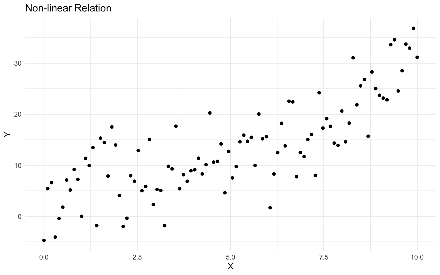
# Fit polynomial regression models
model_linear <- lm(y ~ x, data = nonlinear_data)
model_quad <- lm(y ~ x + I(x^2), data = nonlinear_data)
model_cubic <- lm(y ~ x + I(x^2) + I(x^3), data = nonlinear_data)

# Compare models
modelsummary(
  list(
    "Linear" = model_linear,
    "Quadratic" = model_quad,
    "Cubic" = model_cubic
  ),
  stars = TRUE,
  gof_map = c("nobs", "r.squared", "adj.r.squared", "AIC", "BIC")
)| Linear | Quadratic | Cubic | |
|---|---|---|---|
| + p < 0.1, * p < 0.05, ** p < 0.01, *** p < 0.001 | |||
| (Intercept) | 1.086 | 5.797*** | 2.034 |
| (1.125) | (1.544) | (1.945) | |
| x | 2.478*** | -0.377 | 4.255* |
| (0.194) | (0.714) | (1.693) | |
| I(x^2) | 0.286*** | -0.878* | |
| (0.069) | (0.395) | ||
| I(x^3) | 0.078** | ||
| (0.026) | |||
| Num.Obs. | 100 | 100 | 100 |
| R2 | 0.624 | 0.680 | 0.708 |
| R2 Adj. | 0.620 | 0.674 | 0.699 |
# Plot the fitted curves
ggplot(nonlinear_data, aes(x = x, y = y)) +
  geom_point(alpha = 0.5) +
  geom_smooth(method = "lm", formula = y ~ x, color = "blue", se = FALSE) +
  geom_smooth(method = "lm", formula = y ~ x + I(x^2), color = "red", se = FALSE) +
  geom_smooth(method = "lm", formula = y ~ x + I(x^2) + I(x^3), color = "green", se = FALSE) +
  labs(
    title = "Polynomial Regression Models",
    x = "X",
    y = "Y"
  ) +
  theme_minimal() +
  annotate("text", x = 7, y = 0, label = "Linear", color = "blue") +
  annotate("text", x = 7, y = 5, label = "Quadratic", color = "red") +
  annotate("text", x = 7, y = 10, label = "Cubic", color = "green")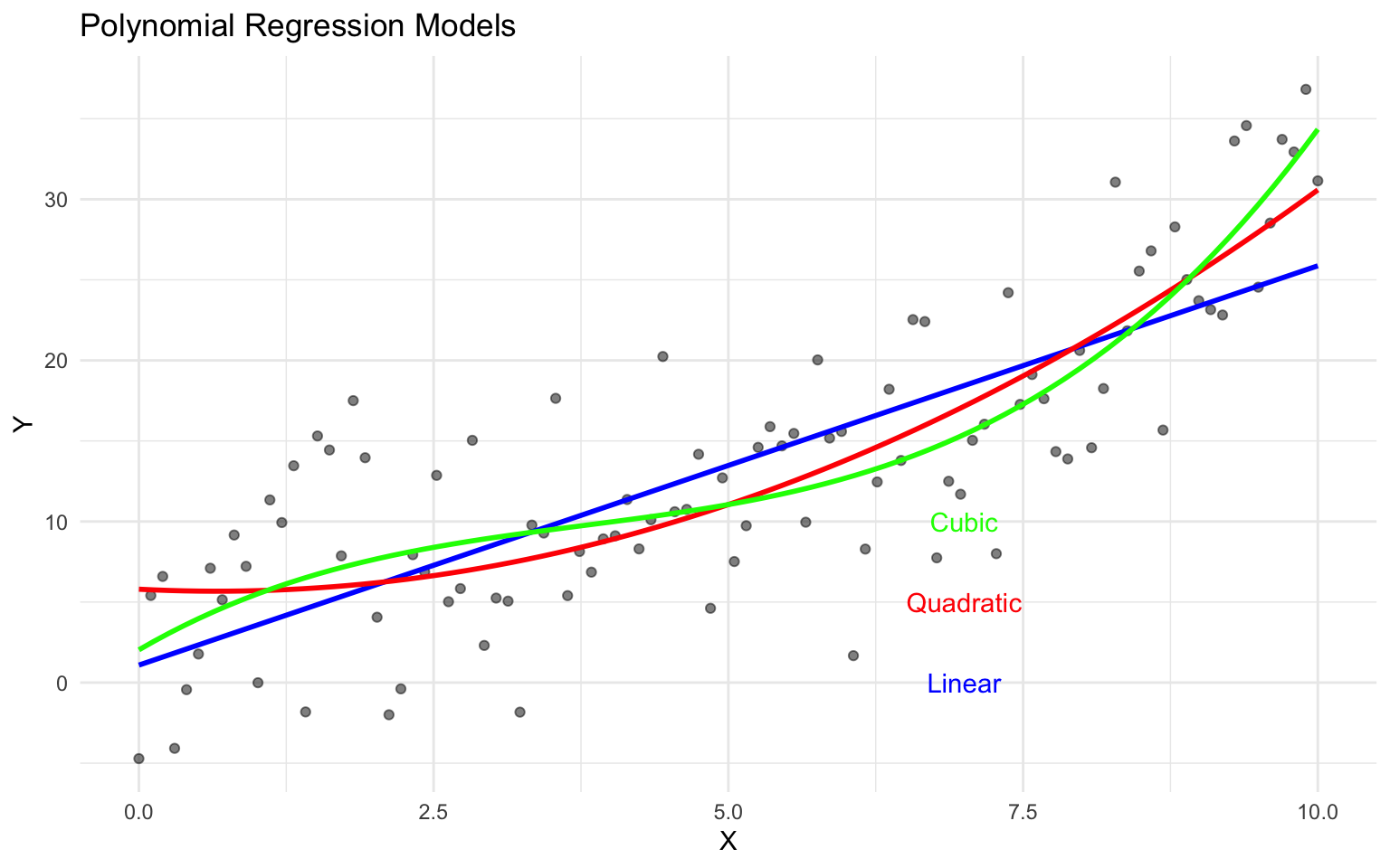
Log Transformations
Log transformations are useful for modeling relations with multiplicative effects or when the data is skewed:
# Create a dataset with a multiplicative relation
set.seed(789)
n <- 100
x <- exp(runif(n, min = 0, max = 3))
y <- 10 * x^0.5 * exp(rnorm(n, mean = 0, sd = 0.2))
log_data <- tibble(x = x, y = y)

# Plot the data
ggplot(log_data, aes(x = x, y = y)) +
  geom_point() +
  labs(
    title = "Multiplicative Relation",
    x = "X",
    y = "Y"
  ) +
  theme_minimal()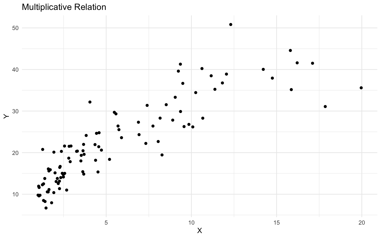
# Fit models with different transformations
model_original <- lm(y ~ x, data = log_data)
model_log_x <- lm(y ~ log(x), data = log_data)
model_log_y <- lm(log(y) ~ x, data = log_data)
model_log_log <- lm(log(y) ~ log(x), data = log_data)

# Compare models
modelsummary(
  list(
    "Original" = model_original,
    "Log X" = model_log_x,
    "Log Y" = model_log_y,
    "Log-Log" = model_log_log
  ),
  stars = TRUE,
  gof_map = c("nobs", "r.squared", "adj.r.squared", "AIC", "BIC")
)| Original | Log X | Log Y | Log-Log | |
|---|---|---|---|---|
| + p < 0.1, * p < 0.05, ** p < 0.01, *** p < 0.001 | ||||
| (Intercept) | 11.655*** | 7.159*** | 2.536*** | 2.300*** |
| (0.791) | (0.907) | (0.042) | (0.041) | |
| x | 1.917*** | 0.084*** | ||
| (0.110) | (0.006) | |||
| log(x) | 10.877*** | 0.505*** | ||
| (0.559) | (0.025) | |||
| Num.Obs. | 100 | 100 | 100 | 100 |
| R2 | 0.757 | 0.795 | 0.681 | 0.803 |
| R2 Adj. | 0.754 | 0.792 | 0.678 | 0.801 |
# Plot the fitted curves
ggplot(log_data, aes(x = x, y = y)) +
  geom_point(alpha = 0.5) +
  geom_smooth(method = "lm", formula = y ~ x, color = "blue", se = FALSE) +
  geom_smooth(method = "lm", formula = y ~ log(x), color = "red", se = FALSE) +
  labs(
    title = "Original vs. Log-Transformed Models",
    x = "X",
    y = "Y"
  ) +
  theme_minimal() +
  annotate("text", x = 15, y = 20, label = "Original", color = "blue") +
  annotate("text", x = 15, y = 30, label = "Log X", color = "red")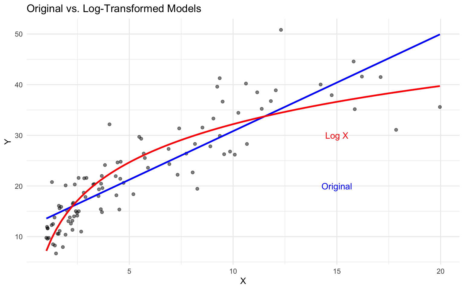
# Plot log-log model
ggplot(log_data, aes(x = log(x), y = log(y))) +
  geom_point(alpha = 0.5) +
  geom_smooth(method = "lm", formula = y ~ x, color = "green", se = FALSE) +
  labs(
    title = "Log-Log Model",
    x = "Log(X)",
    y = "Log(Y)"
  ) +
  theme_minimal()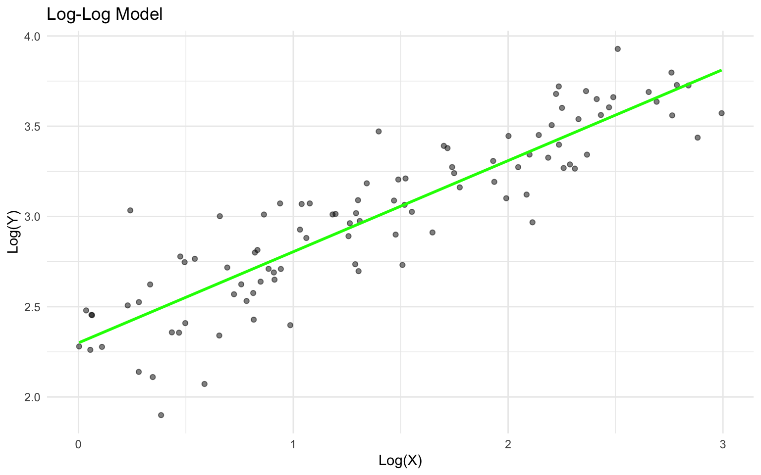
Interpreting Log-Transformed Models
The interpretation of coefficients in log-transformed models depends on the transformation:
- Log-Linear (log(y) ~ x): A one-unit increase in x is associated with a (100 * β)% change in y.
- Linear-Log (y ~ log(x)): A 1% increase in x is associated with a (β/100) unit change in y.
- Log-Log (log(y) ~ log(x)): A 1% increase in x is associated with a β% change in y (elasticity).
In our log-log model, the coefficient is 0.5048107, meaning a 1% increase in x is associated with a 0.5048107% increase in y.
3.10 Interaction Effects
Interaction effects allow the relation between an independent variable and the dependent variable to depend on the value of another independent variable.
Implementing Interaction Effects
Let’s add an interaction term to our car example:
# Create a categorical variable
mtcars$am_factor <- factor(mtcars$am, labels = c("Automatic", "Manual"))

# Fit a model with an interaction
model_interaction <- lm(mpg ~ wt * am_factor, data = mtcars)

# View the model summary
summary(model_interaction)
Call:
lm(formula = mpg ~ wt * am_factor, data = mtcars)

Residuals:
    Min      1Q  Median      3Q     Max
-3.6004 -1.5446 -0.5325  0.9012  6.0909

Coefficients:
                   Estimate Std. Error t value Pr(>|t|)
(Intercept)         31.4161     3.0201  10.402 4.00e-11 ***
wt                  -3.7859     0.7856  -4.819 4.55e-05 ***
am_factorManual     14.8784     4.2640   3.489  0.00162 **
wt:am_factorManual  -5.2984     1.4447  -3.667  0.00102 **
---
Signif. codes:  0 '***' 0.001 '**' 0.01 '*' 0.05 '.' 0.1 ' ' 1

Residual standard error: 2.591 on 28 degrees of freedom
Multiple R-squared:  0.833, Adjusted R-squared:  0.8151
F-statistic: 46.57 on 3 and 28 DF,  p-value: 5.209e-11
Interpreting Interaction Effects
In a model with an interaction term, the effect of one variable depends on the value of another variable:
- The coefficient for
wt(-3.7859075) represents the effect of weight on MPG for automatic transmission cars. - The coefficient for
am_factorManual(14.8784225) represents the difference in MPG between manual and automatic transmission cars when weight is zero (not meaningful in this context). - The coefficient for the interaction term
wt:am_factorManual(-5.2983605) represents the additional effect of weight on MPG for manual transmission cars compared to automatic transmission cars.
Visualizing Interaction Effects
We can visualize the interaction effect:
# Create a plot of the interaction
ggplot(mtcars, aes(x = wt, y = mpg, color = am_factor)) +
  geom_point() +
  geom_smooth(method = "lm", formula = y ~ x, se = TRUE) +
  labs(
    title = "Interaction between Weight and Transmission Type",
    x = "Weight (1000 lbs)",
    y = "Miles per Gallon",
    color = "Transmission"
  ) +
  theme_minimal()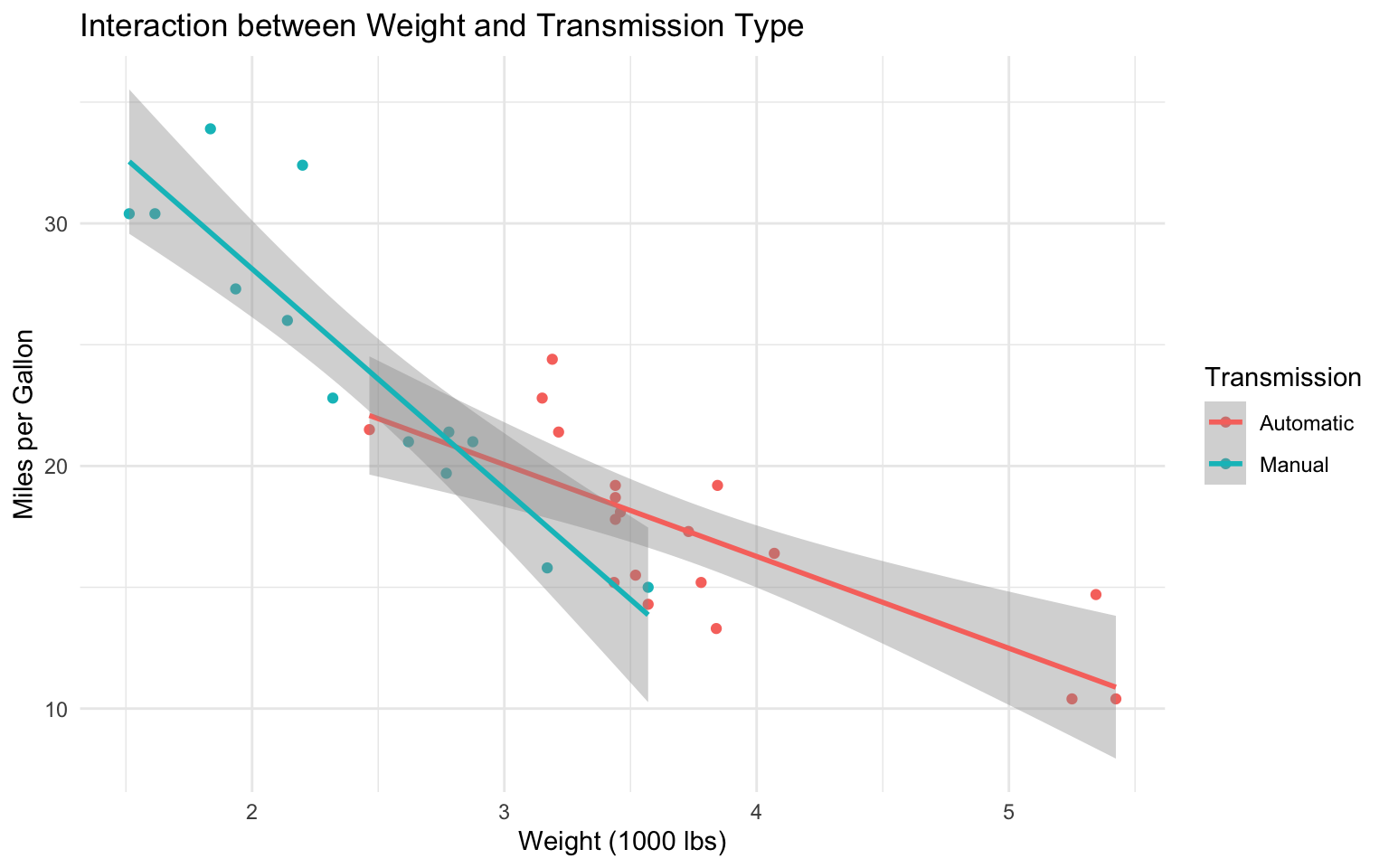
We can also use the ggeffects package to visualize predicted values:
# Visualize predicted values
pred_interaction <- ggpredict(model_interaction, terms = c("wt", "am_factor"))

# Plot predicted values
plot(pred_interaction) +
  labs(
    title = "Predicted MPG by Weight and Transmission Type",
    x = "Weight (1000 lbs)",
    y = "Predicted Miles per Gallon",
    color = "Transmission"
  ) +
  theme_minimal()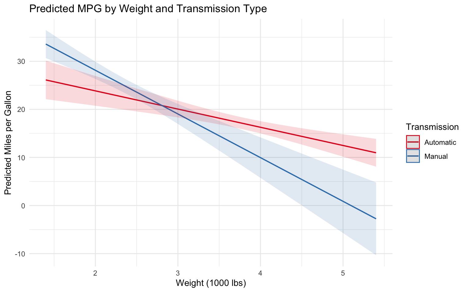
3.11 Marginal Effects
Marginal effects represent the change in the dependent variable associated with a one-unit change in an independent variable, holding other variables constant.
Calculating Marginal Effects
The marginaleffects package provides tools for calculating marginal effects:
# Calculate average marginal effects
mfx <- avg_slopes(model_interaction)
mfx
      Term           Contrast Estimate Std. Error     z Pr(>|z|)    S 2.5 %
 am_factor Manual - Automatic    -2.17      1.419 -1.53    0.127  3.0 -4.95
 wt        dY/dX                 -5.94      0.678 -8.75   <0.001 58.7 -7.27
 97.5 %
  0.613
 -4.609

Type:  response
Visualizing Marginal Effects
We can visualize how marginal effects vary across different values of a variable:
# # Calculate marginal effects of weight at different values
# mfx_by_wt <- slopes(model_interaction, variables = "wt", newdata = datagrid(wt = seq(1.5, 5.5, by = 0.5), am_factor = "Automatic"))
#
# # Plot marginal effects
# plot_cme(mfx_by_wt) +
#   labs(
#     title = "Marginal Effect of Weight on MPG",
#     subtitle = "For Automatic Transmission Cars",
#     x = "Weight (1000 lbs)",
#     y = "Marginal Effect on MPG"
#   ) +
#   theme_minimal()
3.12 Business Case Study: Sales Response Modeling
Let’s apply regression analysis to a business case study on sales response modeling.
The Scenario
You’re a marketing analyst at a retail company. You’ve been asked to analyze the relation between advertising spending across different channels (TV, radio, and online) and sales. The goal is to understand the effectiveness of each channel and optimize the marketing budget allocation.
The Data
# Create a simulated advertising dataset
set.seed(123)
n <- 200

# Generate advertising spending
tv_spend <- runif(n, min = 5, max = 50)
radio_spend <- runif(n, min = 1, max = 20)
online_spend <- runif(n, min = 10, max = 40)

# Generate sales with diminishing returns and interaction effects
sales <- 10 + 3 * log(tv_spend) + 2 * sqrt(radio_spend) + 1.5 * online_spend +
         0.1 * sqrt(tv_spend * radio_spend) + 0.05 * sqrt(tv_spend * online_spend) +
         rnorm(n, mean = 0, sd = 5)

# Create a data frame
advertising_data <- tibble(
  tv_spend = tv_spend,
  radio_spend = radio_spend,
  online_spend = online_spend,
  sales = sales
)

# View the data
glimpse(advertising_data)
Rows: 200
Columns: 4
$ tv_spend <dbl> 17.940988, 40.473731, 23.403961, 44.735783, 47.321028, 7.…
$ radio_spend <dbl> 5.535795, 19.284820, 12.425949, 10.785565, 8.648894, 17.7…
$ online_spend <dbl> 39.58163, 14.11202, 37.15929, 27.28906, 21.86347, 23.4940…
$ sales <dbl> 81.49215, 51.27820, 80.73489, 67.58520, 61.69338, 62.9376…Exploratory Data Analysis
Let’s start by exploring the relations in the data:
# Scatter plot matrix
pairs(advertising_data)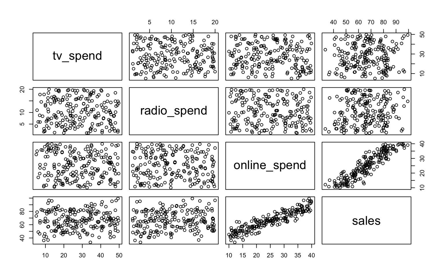
# Correlation matrix
cor(advertising_data)
tv_spend radio_spend online_spend sales
tv_spend 1.00000000 -0.05250087 -0.06925880 0.04543969
radio_spend -0.05250087 1.00000000 -0.07378403 0.10309680
online_spend -0.06925880 -0.07378403 1.00000000 0.91240242
sales 0.04543969 0.10309680 0.91240242 1.00000000# Visualize relations
p1 <- ggplot(advertising_data, aes(x = tv_spend, y = sales)) +
geom_point(alpha = 0.5) +
geom_smooth(method = "loess", se = FALSE) +
labs(
title = "Sales vs. TV Advertising",
x = "TV Advertising Spend ($1000s)",
y = "Sales ($1000s)"
) +
theme_minimal()
p2 <- ggplot(advertising_data, aes(x = radio_spend, y = sales)) +
geom_point(alpha = 0.5) +
geom_smooth(method = "loess", se = FALSE) +
labs(
title = "Sales vs. Radio Advertising",
x = "Radio Advertising Spend ($1000s)",
y = "Sales ($1000s)"
) +
theme_minimal()
p3 <- ggplot(advertising_data, aes(x = online_spend, y = sales)) +
geom_point(alpha = 0.5) +
geom_smooth(method = "loess", se = FALSE) +
labs(
title = "Sales vs. Online Advertising",
x = "Online Advertising Spend ($1000s)",
y = "Sales ($1000s)"
) +
theme_minimal()
# Combine plots
gridExtra::grid.arrange(p1, p2, p3, ncol = 3)`geom_smooth()` using formula = 'y ~ x'
`geom_smooth()` using formula = 'y ~ x'
`geom_smooth()` using formula = 'y ~ x'
Model Building
Let’s build and compare several models:
# Linear model
model_linear <- lm(sales ~ tv_spend + radio_spend + online_spend, data = advertising_data)

# Model with transformations
model_trans <- lm(sales ~ log(tv_spend) + sqrt(radio_spend) + online_spend, data = advertising_data)

# Model with interactions
model_interact <- lm(sales ~ log(tv_spend) + sqrt(radio_spend) + online_spend +
                           I(sqrt(tv_spend * radio_spend)) + I(sqrt(tv_spend * online_spend)),
                    data = advertising_data)

# Compare models
modelsummary(
  list(
    "Linear" = model_linear,
    "Transformed" = model_trans,
    "Interaction" = model_interact
  ),
  stars = TRUE,
  gof_map = c("nobs", "r.squared", "adj.r.squared", "AIC", "BIC")
)| Linear | Transformed | Interaction | |
|---|---|---|---|
| + p < 0.1, * p < 0.05, ** p < 0.01, *** p < 0.001 | |||
| (Intercept) | 19.545*** | 9.796*** | 13.997+ |
| (1.614) | (2.833) | (8.462) | |
| tv_spend | 0.138*** | ||
| (0.029) | |||
| radio_spend | 0.457*** | ||
| (0.065) | |||
| online_spend | 1.526*** | 1.523*** | 1.525*** |
| (0.041) | (0.041) | (0.141) | |
| log(tv_spend) | 3.229*** | 1.914 | |
| (0.684) | (3.318) | ||
| sqrt(radio_spend) | 2.614*** | 1.619 | |
| (0.383) | (1.525) | ||
| I(sqrt(tv_spend * radio_spend)) | 0.197 | ||
| (0.291) | |||
| I(sqrt(tv_spend * online_spend)) | -0.002 | ||
| (0.261) | |||
| Num.Obs. | 200 | 200 | 200 |
| R2 | 0.876 | 0.875 | 0.876 |
| R2 Adj. | 0.874 | 0.873 | 0.873 |
Model Diagnostics
Let’s check the assumptions of our best model:
# Check model assumptions
check_model(model_interact)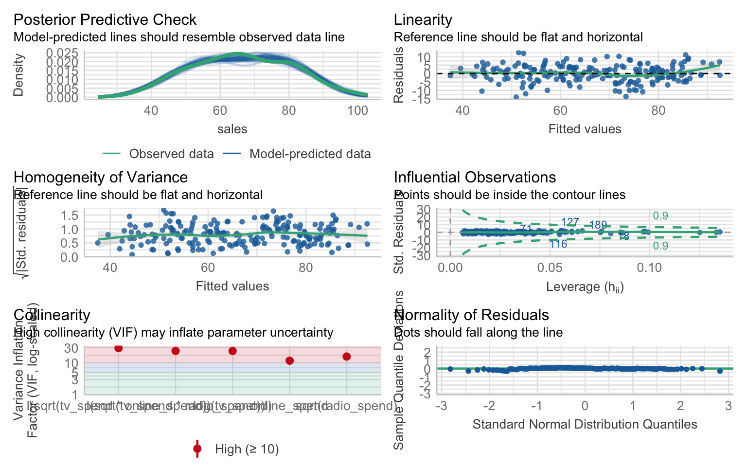
Calculating Elasticities
In marketing, elasticities are often used to measure the responsiveness of sales to changes in advertising spending:
# Calculate elasticities at the mean
mean_values <- colMeans(advertising_data)

# TV elasticity
tv_elasticity <- coef(model_interact)[2] * (mean_values["tv_spend"] / mean_values["sales"])

# Radio elasticity
radio_elasticity <- coef(model_interact)[3] * (0.5 / sqrt(mean_values["radio_spend"])) * (mean_values["radio_spend"] / mean_values["sales"])

# Online elasticity
online_elasticity <- coef(model_interact)[4] * (mean_values["online_spend"] / mean_values["sales"])

# Create a table of elasticities
elasticities <- tibble(
  Channel = c("TV", "Radio", "Online"),
  Elasticity = c(tv_elasticity, radio_elasticity, online_elasticity)
)

elasticities
# A tibble: 3 × 2
Channel Elasticity
<chr> <dbl>
1 TV 0.802
2 Radio 0.0391
3 Online 0.576 Optimal Budget Allocation
Based on the elasticities, we can determine the optimal budget allocation:
# Total budget
total_budget <- sum(mean_values[c("tv_spend", "radio_spend", "online_spend")])

# Optimal allocation based on elasticities
optimal_allocation <- elasticities %>%
  mutate(
    Proportion = Elasticity / sum(Elasticity),
    Optimal_Budget = Proportion * total_budget
  )

optimal_allocation
# A tibble: 3 × 4
Channel Elasticity Proportion Optimal_Budget
<chr> <dbl> <dbl> <dbl>
1 TV 0.802 0.566 35.7
2 Radio 0.0391 0.0276 1.74
3 Online 0.576 0.407 25.7 Visualizing the Results
Let’s visualize the current vs. optimal budget allocation:
# Current allocation
current_allocation <- tibble(
  Channel = c("TV", "Radio", "Online"),
  Budget = c(mean_values["tv_spend"], mean_values["radio_spend"], mean_values["online_spend"]),
  Allocation = "Current"
)

# Combine with optimal allocation
allocation_comparison <- bind_rows(
  current_allocation,
  optimal_allocation %>% select(Channel, Budget = Optimal_Budget) %>% mutate(Allocation = "Optimal")
)

# Plot the comparison
ggplot(allocation_comparison, aes(x = Channel, y = Budget, fill = Allocation)) +
  geom_bar(stat = "identity", position = "dodge") +
  labs(
    title = "Current vs. Optimal Budget Allocation",
    x = NULL,
    y = "Budget ($1000s)"
  ) +
  theme_minimal()
Business Recommendations
Based on our analysis, we can provide the following recommendations:
- Budget Reallocation: Shift some budget from online advertising to TV and radio advertising, as they have higher elasticities.
- Diminishing Returns: Be aware of diminishing returns, especially for TV advertising (log transformation).
- Synergy Effects: Leverage the positive interaction effects between TV and radio advertising.
- Continuous Monitoring: Regularly update the model as new data becomes available to ensure optimal budget allocation.
3.13 Exercises
Exercise 1: Simple and Multiple Regression
Using the mtcars dataset:
- Fit a simple linear regression model with
mpgas the dependent variable andhpas the independent variable. - Fit a multiple regression model with
mpgas the dependent variable andhp,wt, andqsecas independent variables. - Compare the two models using appropriate statistical tests and criteria.
- Interpret the coefficients of the multiple regression model in business terms.
- Check the assumptions of the multiple regression model and address any violations.
Exercise 2: Fixed Effects Regression
Using the panel data example from this chapter:
- Create a new panel dataset with firms, years, and additional variables of your choice.
- Fit a pooled OLS model, a firm fixed effects model, and a two-way fixed effects model.
- Compare the models and interpret the results.
- Explain why fixed effects might be important in this context.
- Visualize the estimated fixed effects and discuss their implications.
Exercise 3: Non-linear Regression
Using a dataset of your choice:
- Identify a relation that appears to be non-linear.
- Fit at least three different non-linear models (e.g., polynomial, log-transformed).
- Compare the models using appropriate criteria.
- Interpret the results of the best-fitting model.
- Create visualizations to illustrate the non-linear relation.
Exercise 4: Business Application
You are a business analyst at a company that wants to understand the factors affecting employee productivity:
- Create a simulated dataset with variables such as hours worked, experience, training, team size, and productivity.
- Explore the relations in the data using appropriate visualizations.
- Fit multiple regression models to identify the key drivers of productivity.
- Check model assumptions and address any issues.
- Provide business recommendations based on your analysis.
Exercise 5: Multicollinearity Analysis
Using a dataset of your choice:
- Create a regression model with potential multicollinearity issues.
- Calculate and interpret VIF values for the independent variables.
- Apply at least two different methods to address multicollinearity.
- Compare the original and modified models.
- Discuss the trade-offs between addressing multicollinearity and maintaining model interpretability.
3.14 Summary
In this chapter, we’ve covered the fundamentals of regression analysis for business applications. We’ve learned how to:
- Implement and interpret simple and multiple linear regression models
- Use fixed effects regression for panel data
- Apply non-linear regression techniques
- Perform model diagnostics to validate regression assumptions
- Identify and address multicollinearity using VIF analysis
- Compare and select models based on statistical criteria
- Visualize regression results for business presentations
- Calculate and interpret marginal effects and elasticities
- Apply regression analysis to business problems like sales response modeling
These skills provide a solid foundation for predictive modeling in business contexts. By understanding the relations between variables and quantifying their effects, you can make more informed business decisions and develop effective strategies.
In the next chapter, we’ll build on these skills to explore classification models, which are useful for predicting categorical outcomes such as customer churn, credit default, and purchase decisions.
3.15 References
- Fox, J. (2015). Applied Regression Analysis and Generalized Linear Models. SAGE Publications.
- Wooldridge, J. M. (2010). Econometric Analysis of Cross Section and Panel Data. MIT Press.
- James, G., Witten, D., Hastie, T., & Tibshirani, R. (2021). An Introduction to Statistical Learning with Applications in R. Springer.
- Bergeaud, A., & Vermare, L. (2022). The fixest R Package: Fast Fixed-Effects Estimation. https://cran.r-project.org/web/packages/fixest/vignettes/fixest_walkthrough.html
- Huntington-Klein, N. (2021). The Effect: An Introduction to Research Design and Causality. https://theeffectbook.net/ch-FixedEffects.html
- Belsley, D. A., Kuh, E., & Welsch, R. E. (1980). Regression Diagnostics: Identifying Influential Data and Sources of Collinearity. Wiley.