# Install required packages if not already installed
if (!require("tidyverse")) install.packages("tidyverse")
if (!require("tidymodels")) install.packages("tidymodels")
if (!require("ranger")) install.packages("ranger")
if (!require("xgboost")) install.packages("xgboost")
if (!require("glmnet")) install.packages("glmnet")
if (!require("vip")) install.packages("vip")
if (!require("doParallel")) install.packages("doParallel")
if (!require("finetune")) install.packages("finetune")
if (!require("skimr")) install.packages("skimr")
if (!require("tictoc")) install.packages("tictoc")5 🎯 Machine Learning (ML) I: Model Selection 🔬 & Hyperparameter Tuning 🧪
5.1 Learning Objectives
By the end of this chapter, you will be able to:
- Understand the principles of model selection and hyperparameter tuning for predicting greenhouse gas emissions
- Implement cross-validation for robust model evaluation with panel data
- Apply grid search and random search for hyperparameter optimization
- Use the tidymodels framework for streamlined machine learning workflows
- Evaluate model performance using appropriate metrics
- Avoid overfitting through proper validation techniques
- Compare and select models based on business requirements
- Create reproducible machine learning pipelines for sustainability analytics
5.2 Prerequisites
For this chapter, you’ll need:
- R and RStudio installed on your computer
- Understanding of data manipulation with dplyr
- Basic knowledge of data visualization with ggplot2
- Familiarity with regression analysis
- The following R packages installed:
# Load required packages
library(tidyverse)      # For data manipulation and visualization
library(tidymodels)     # For modeling framework
library(ranger)         # For random forests
library(xgboost)        # For gradient boosting
library(glmnet)         # For regularized regression
library(vip)            # For variable importance plots
library(doParallel)     # For parallel processing
library(finetune)       # For advanced hyperparameter tuning
library(skimr)          # For data summaries
library(tictoc)         # For timing code
library(bonsai)         # For LightGBM
library(rules)          # For Cubist algorithm
library(embed)          # For embeddings
library(themis)         # For balancing

# Set seed for reproducibility
set.seed(12345)
5.3 Introduction to Predicting Greenhouse Gas Emissions and SBTI Targets
In this chapter, we’ll work with a dataset related to corporate sustainability, specifically focusing on greenhouse gas (GHG) emissions and Science-Based Targets Initiative (SBTI) commitments. The Science-Based Targets initiative is a collaboration that helps companies set ambitious emissions reduction targets consistent with limiting global warming to well below 2°C above pre-industrial levels.
Our primary task is to predict a company’s greenhouse gas emissions (log_scope_1_ghg_emissions) based on various financial and sustainability indicators. Additionally, we’ll explore what factors are associated with companies committing to SBTI targets (sb_ti_committed).
Understanding the Data
Let’s first load and examine our dataset:
# For demonstration purposes, we'll create a sample of the data
# In a real scenario, you would load the data from a file or database
# Create a sample dataset based on the structure provided
set.seed(12345)
n_obs <- 1000  # Using a smaller sample for efficiency

# Generate sample data
ml_data <- tibble(
  log_scope_1_ghg_emissions = rnorm(n_obs, mean = 11.1, sd = 3.17),
  sb_ti_committed = sample(c(0, 1), n_obs, replace = TRUE, prob = c(0.93, 0.07)),
  management_incentives = sample(c(0, 1, NA), n_obs, replace = TRUE, prob = c(0.64, 0.09, 0.27)),
  esg_audit = sample(c(0, 1, NA), n_obs, replace = TRUE, prob = c(0.62, 0.38, 0.001)),
  climate_change_policy = sample(c(0, 1, NA), n_obs, replace = TRUE, prob = c(0.31, 0.68, 0.01)),
  log_market_capitalization = rnorm(n_obs, mean = 23.3, sd = 1.43),
  log_net_sales = rnorm(n_obs, mean = 22.6, sd = 1.39),
  price_to_book_ratio = rexp(n_obs, rate = 1/5.21),
  log_total_assets = rnorm(n_obs, mean = 23.3, sd = 1.47),
  gvkey = sample(1:1039, n_obs, replace = TRUE)
)

# Convert categorical variables to factors
ml_data <- ml_data %>%
  mutate(across(c(sb_ti_committed, management_incentives, esg_audit, climate_change_policy),
                ~factor(., levels = c(0, 1))),
         gvkey = factor(gvkey))

# Display data structure
glimpse(ml_data)
Rows: 1,000
Columns: 10
$ log_scope_1_ghg_emissions <dbl> 12.956126, 13.349007, 10.753508, 9.662414, 1…
$ sb_ti_committed <fct> 1, 0, 0, 0, 0, 0, 0, 0, 0, 1, 0, 0, 0, 0, 0,…
$ management_incentives <fct> 0, NA, 0, NA, NA, NA, NA, 0, 0, NA, 0, 0, 0,…
$ esg_audit <fct> 0, 1, 1, 0, 0, 1, 1, 0, 1, 1, 0, 1, 1, 0, 0,…
$ climate_change_policy <fct> 1, 1, 0, 1, 1, 0, 1, 0, 1, 1, 0, 1, 1, 0, 1,…
$ log_market_capitalization <dbl> 24.02915, 22.27703, 22.72010, 23.28209, 24.8…
$ log_net_sales <dbl> 21.15066, 22.34431, 22.84918, 21.67058, 21.2…
$ price_to_book_ratio <dbl> 9.71222598, 0.72187204, 8.86182428, 21.03081…
$ log_total_assets <dbl> 24.09063, 23.65575, 24.02548, 24.19977, 24.7…
$ gvkey <fct> 292, 188, 667, 1012, 272, 897, 312, 42, 351,…# Summary statistics
skim(ml_data)| Name | ml_data |
| Number of rows | 1000 |
| Number of columns | 10 |
| _______________________ | |
| Column type frequency: | |
| factor | 5 |
| numeric | 5 |
| ________________________ | |
| Group variables | None |
Variable type: factor
| skim_variable | n_missing | complete_rate | ordered | n_unique | top_counts |
|---|---|---|---|---|---|
| sb_ti_committed | 0 | 1.00 | FALSE | 2 | 0: 935, 1: 65 |
| management_incentives | 267 | 0.73 | FALSE | 2 | 0: 651, 1: 82 |
| esg_audit | 1 | 1.00 | FALSE | 2 | 0: 633, 1: 366 |
| climate_change_policy | 8 | 0.99 | FALSE | 2 | 1: 690, 0: 302 |
| gvkey | 0 | 1.00 | FALSE | 645 | 623: 6, 209: 5, 344: 5, 660: 5 |
Variable type: numeric
| skim_variable | n_missing | complete_rate | mean | sd | p0 | p25 | p50 | p75 | p100 | hist |
|---|---|---|---|---|---|---|---|---|---|---|
| log_scope_1_ghg_emissions | 0 | 1 | 11.25 | 3.17 | 2.29 | 9.21 | 11.25 | 13.28 | 21.66 | ▁▅▇▃▁ |
| log_market_capitalization | 0 | 1 | 23.32 | 1.36 | 18.50 | 22.43 | 23.28 | 24.23 | 27.01 | ▁▂▇▆▁ |
| log_net_sales | 0 | 1 | 22.59 | 1.43 | 17.20 | 21.67 | 22.67 | 23.51 | 27.14 | ▁▃▇▅▁ |
| price_to_book_ratio | 0 | 1 | 5.40 | 5.34 | 0.01 | 1.54 | 3.68 | 7.59 | 39.65 | ▇▂▁▁▁ |
| log_total_assets | 0 | 1 | 23.37 | 1.49 | 18.62 | 22.35 | 23.40 | 24.39 | 27.36 | ▁▃▇▆▁ |
Data Description
Our dataset contains the following variables:
- log_scope_1_ghg_emissions: Logarithm of Scope 1 greenhouse gas emissions (direct emissions from owned or controlled sources)
- sb_ti_committed: Whether the company has committed to Science-Based Targets (0 = No, 1 = Yes)
- management_incentives: Whether management compensation is linked to ESG/sustainability performance (0 = No, 1 = Yes)
- esg_audit: Whether the company conducts ESG audits (0 = No, 1 = Yes)
- climate_change_policy: Whether the company has a climate change policy (0 = No, 1 = Yes)
- log_market_capitalization: Logarithm of market capitalization (company size)
- log_net_sales: Logarithm of net sales (revenue)
- price_to_book_ratio: Price-to-book ratio (market value relative to book value)
- log_total_assets: Logarithm of total assets
- gvkey: Company identifier
Our primary task is to predict log_scope_1_ghg_emissions using the other variables as predictors.
5.4 Data Preparation
Before building our models, we need to prepare the data. This includes adding random noise features (for feature importance testing), splitting the data into training and testing sets, and setting up cross-validation.
# Add random noise features (for feature importance testing)
for (i in 1:4) {
  column <- tibble(sample(1:100, nrow(ml_data), replace = TRUE))
  names(column) <- paste0("random", i)
  ml_data <- cbind(ml_data, column)
}

# Train-test split (group-based sampling by company)
train_test_split <- group_initial_split(ml_data, group = gvkey, prop = 0.8)
train_data <- training(train_test_split)
test_data <- testing(train_test_split)

# Set up cross-validation (3-fold, grouped by company)
train_resamples <- group_vfold_cv(
  train_data,
  group = gvkey,
  v = 3,
  repeats = 1
)

# Display the resampling structure
train_resamples
# Group 3-fold cross-validation
# A tibble: 3 × 2
splits id
<list> <chr>
1 <split [531/269]> Resample1
2 <split [540/260]> Resample2
3 <split [529/271]> Resample3Why Group-Based Splitting?
In this dataset, we have multiple observations per company (identified by gvkey). Using group-based splitting ensures that all observations from the same company are either in the training set or the testing set, but not both. This is crucial for several reasons:
Preventing Data Leakage: If observations from the same company appear in both training and testing sets, the model might “memorize” company-specific patterns rather than learning generalizable relations.
Realistic Evaluation: In practice, we often want to predict emissions for companies that weren’t in our training data. Group-based splitting simulates this scenario.
Independence Assumption: Many statistical models assume independence between observations. Observations from the same company are likely correlated, violating this assumption.
5.5 Feature Engineering
Next, we’ll create a recipe for preprocessing our data. This includes handling missing values, encoding categorical variables, and other transformations.
# Base recipe (feature engineering)
ml_recipe <- recipe(log_scope_1_ghg_emissions ~ ., data = train_data) %>%
  update_role(gvkey, new_role = "id") %>%  # Preserve ID columns
  step_novel(all_nominal_predictors()) %>%  # Handle new levels in categorical variables
  step_unknown(all_nominal(), new_level = "unknown") %>%  # Handle unknown levels
  step_dummy(all_nominal_predictors(), one_hot = TRUE) %>%  # One-hot encode categorical variables
  step_impute_median(all_numeric_predictors()) %>%  # Impute missing numeric values with median
  step_zv(all_predictors())  # Remove zero-variance predictors

# Print the recipe
ml_recipe
── Recipe ──────────────────────────────────────────────────────────────────────── Inputs Number of variables by roleoutcome: 1
predictor: 12
id: 1── Operations • Novel factor level assignment for: all_nominal_predictors()• Unknown factor level assignment for: all_nominal()• Dummy variables from: all_nominal_predictors()• Median imputation for: all_numeric_predictors()• Zero variance filter on: all_predictors()Understanding the Recipe Steps
update_role(gvkey, new_role = “id”): This tells the recipe that
gvkeyis an identifier, not a predictor.step_novel(all_nominal_predictors()): This handles new levels in categorical variables that might appear in the test set but not in the training set.
step_unknown(all_nominal(), new_level = “unknown”): This handles unknown levels in categorical variables.
step_dummy(all_nominal_predictors(), one_hot = TRUE): This converts categorical variables to dummy variables using one-hot encoding.
step_impute_median(all_numeric_predictors()): This imputes missing numeric values with the median.
step_zv(all_predictors()): This removes predictors with zero variance, which don’t provide any information for prediction.
5.6 Model Specification
Now, let’s define the models we want to evaluate. We’ll start with a gradient boosting model (XGBoost) and then add more models for comparison.
# XGBoost model specification with tunable parameters
boost_tree_tune_spec <-
  boost_tree(mode = "regression",
    engine = "xgboost",
    mtry = tune(),
    trees = 1000,
    min_n = tune(),
    tree_depth = tune(),
    learn_rate = tune(),
    loss_reduction = tune(),
    sample_size = tune())

# LightGBM model specification
lightGBM_tune_spec <-
  boost_tree(mode = "regression",
    engine = "lightgbm",
    mtry = tune(),
    trees = 1000,
    min_n = tune(),
    tree_depth = tune(),
    learn_rate = tune(),
    loss_reduction = tune(),
    sample_size = tune())

# Neural network model specification
mlp_tune_spec <-
  mlp(mode = "regression",
    engine = "nnet",
    hidden_units = tune(),
    penalty = tune(),
    epochs = tune())

# Regularized regression model specification (Elastic Net)
glmnet_tune_spec <-
  linear_reg(mode="regression",
    engine = "glmnet",
    penalty = tune(),
    mixture = tune())

# K-nearest neighbors model specification
knn_tune_spec <-
  nearest_neighbor(mode = "regression",
    engine = "kknn",
    neighbors = tune(),
    weight_func = tune(),
    dist_power = tune())

# Random forest model specification
rand_forest_tune_spec <-
  rand_forest(mode="regression",
    engine = "ranger",
    mtry = tune(),
    trees = 1000,
    min_n = tune())

# Linear SVM model specification
svm_linear_tune_spec <-
  svm_linear(mode = "regression",
    engine = "LiblineaR",
    cost = tune(),
    margin = tune())

# Polynomial SVM model specification
svm_poly_tune_spec <-
  svm_poly(mode = "regression",
    engine = "kernlab",
    cost = tune(),
    degree = tune(),
    scale_factor = tune(),
    margin = tune())

# Radial basis function SVM model specification
svm_rbf_tune_spec <-
  svm_rbf(mode = "regression",
    engine = "kernlab",
    cost = tune(),
    rbf_sigma = tune(),
    margin = tune())
Understanding Model Hyperparameters
Each model has its own set of hyperparameters that need to be tuned:
- Gradient Boosting (XGBoost and LightGBM):
mtry: Number of predictors randomly sampled at each splittrees: Number of trees in the ensemblemin_n: Minimum number of observations in a nodetree_depth: Maximum depth of treeslearn_rate: Learning rate (shrinkage)loss_reduction: Minimum loss reduction to split a nodesample_size: Proportion of data used for training each tree
- Neural Network:
hidden_units: Number of units in the hidden layerpenalty: Weight decay (regularization)epochs: Number of training iterations
- Regularized Regression (Elastic Net):
penalty: Regularization strengthmixture: Mixing parameter (0 = ridge, 1 = lasso)
- K-Nearest Neighbors:
neighbors: Number of neighborsweight_func: Weighting functiondist_power: Power parameter for Minkowski distance
- Random Forest:
mtry: Number of predictors randomly sampled at each splittrees: Number of trees in the forestmin_n: Minimum number of observations in a node
- Support Vector Machines:
cost: Cost of constraint violationmargin: Epsilon in the epsilon-insensitive loss functiondegree: Degree of polynomial kernel (for polynomial SVM)scale_factor: Scale factor for polynomial kernel (for polynomial SVM)rbf_sigma: Inverse kernel width (for radial basis function SVM)
5.7 Creating Workflow Sets
Now, let’s create workflow sets that combine our preprocessing recipe with different models. This allows us to systematically evaluate multiple modeling approaches.
# Define workflow set for tree-based models
tree_workflows <-
  workflow_set(preproc = list(recipe = ml_recipe),
               models = list(xgboost = boost_tree_tune_spec,
                            lightGBM = lightGBM_tune_spec,
                            rand_forest = rand_forest_tune_spec),
               cross = TRUE)

# Define workflow set for other models
other_workflows <-
  workflow_set(preproc = list(recipe = ml_recipe),
               models = list(glmnet = glmnet_tune_spec,
                            knn = knn_tune_spec,
                            nnet = mlp_tune_spec,
                            svm_linear = svm_linear_tune_spec,
                            svm_poly = svm_poly_tune_spec,
                            svm_rbf = svm_rbf_tune_spec),
               cross = TRUE)

# Combine all workflows
tune_workflows <- bind_rows(tree_workflows, other_workflows)

# Display the workflow set
tune_workflows
# A workflow set/tibble: 9 × 4
wflow_id info option result
<chr> <list> <list> <list>
1 recipe_xgboost <tibble [1 × 4]> <opts[0]> <list [0]>
2 recipe_lightGBM <tibble [1 × 4]> <opts[0]> <list [0]>
3 recipe_rand_forest <tibble [1 × 4]> <opts[0]> <list [0]>
4 recipe_glmnet <tibble [1 × 4]> <opts[0]> <list [0]>
5 recipe_knn <tibble [1 × 4]> <opts[0]> <list [0]>
6 recipe_nnet <tibble [1 × 4]> <opts[0]> <list [0]>
7 recipe_svm_linear <tibble [1 × 4]> <opts[0]> <list [0]>
8 recipe_svm_poly <tibble [1 × 4]> <opts[0]> <list [0]>
9 recipe_svm_rbf <tibble [1 × 4]> <opts[0]> <list [0]>Understanding Workflow Sets
A workflow set combines preprocessing recipes with model specifications. This allows us to:
Systematically Evaluate Models: We can compare different models using the same preprocessing steps and evaluation metrics.
Streamline Tuning: We can tune multiple models with a single function call.
Ensure Consistency: All models are evaluated on the same resamples, making comparisons fair.
5.8 Parallel Processing Setup
Hyperparameter tuning can be computationally intensive. To speed up the process, we’ll use parallel processing.
# Parallel processing setup
cl <- makePSOCKcluster(8)  # Create clusters (adjust based on your computer's capabilities)
registerDoParallel(cl)
getDoParWorkers()  # Check number of workers

# When done, remember to stop the cluster
# stopCluster(cl)
# registerDoSEQ()
5.9 Model Tuning
Now, let’s tune our models using the workflow set and cross-validation.
# Tune all models in the workflow set
tune_workflows_models <-
  tune_workflows %>%
  workflow_map("tune_grid",  # Specify tuning function
               resamples = train_resamples,  # Resampling scheme
               grid = 25,  # Grid size (25 combinations per model)
               metrics = metric_set(rmse, rsq, mae),  # Evaluation metrics
               verbose = TRUE)

# Stop parallel processing
# stopCluster(cl)
# registerDoSEQ()
# gc()  # Run garbage collection to clear memory
For demonstration purposes, we’ll create a simulated result:
# Simulated results for demonstration
set.seed(12345)
model_names <- c("recipe_xgboost", "recipe_lightGBM", "recipe_rand_forest",
                "recipe_glmnet", "recipe_knn", "recipe_nnet",
                "recipe_svm_linear", "recipe_svm_poly", "recipe_svm_rbf")

# Create simulated metrics
sim_metrics <- tibble(
  wflow_id = rep(model_names, each = 3),
  .metric = rep(c("rmse", "rsq", "mae"), times = length(model_names)),
  mean = case_when(
    .metric == "rmse" ~ runif(length(model_names) * 3, 0.8, 2.5),
    .metric == "rsq" ~ runif(length(model_names) * 3, 0.6, 0.9),
    .metric == "mae" ~ runif(length(model_names) * 3, 0.6, 2.0)
  ),
  n = rep(3, length(model_names) * 3),
  std_err = runif(length(model_names) * 3, 0.05, 0.2),
  rank = case_when(
    .metric == "rmse" ~ rank(mean),
    .metric == "rsq" ~ rank(-mean),
    .metric == "mae" ~ rank(mean)
  ),
  model = case_when(
    str_detect(wflow_id, "xgboost") ~ "boost_tree",
    str_detect(wflow_id, "lightGBM") ~ "boost_tree",
    str_detect(wflow_id, "rand_forest") ~ "rand_forest",
    str_detect(wflow_id, "glmnet") ~ "linear_reg",
    str_detect(wflow_id, "knn") ~ "nearest_neighbor",
    str_detect(wflow_id, "nnet") ~ "mlp",
    str_detect(wflow_id, "svm_linear") ~ "svm_linear",
    str_detect(wflow_id, "svm_poly") ~ "svm_poly",
    str_detect(wflow_id, "svm_rbf") ~ "svm_rbf"
  ),
  .config = paste0("Preprocessor1_Model", sample(1:5, length(model_names) * 3, replace = TRUE))
)

# Simulate a workflow set results object
# This is a simplified version for demonstration
tune_workflows_models <- list(
  metrics = sim_metrics
)

# Function to extract metrics from our simulated object
rank_results <- function(object, rank_metric = "rmse", select_best = FALSE) {
  if (select_best) {
    object$metrics %>%
      group_by(wflow_id, .metric) %>%
      slice_min(order_by = ifelse(.metric == "rsq", -mean, mean), n = 1) %>%
      ungroup()
  } else {
    object$metrics
  }
}

collect_metrics <- function(object) {
  object$metrics
}
5.10 Evaluating Model Performance
Let’s evaluate the performance of our models.
# Rank models by MAE
rank_results(tune_workflows_models, rank_metric = "mae") %>%
  filter(.metric == "mae") %>%
  arrange(rank)
# A tibble: 9 × 8
wflow_id .metric mean n std_err rank model .config
<chr> <chr> <dbl> <dbl> <dbl> <dbl> <chr> <chr>
1 recipe_svm_linear mae 0.668 3 0.143 3 svm_linear Preproc…
2 recipe_glmnet mae 0.907 3 0.0618 11 linear_reg Preproc…
3 recipe_lightGBM mae 0.931 3 0.174 12 boost_tree Preproc…
4 recipe_nnet mae 1.31 3 0.0643 14 mlp Preproc…
5 recipe_knn mae 1.44 3 0.127 17 nearest_neighbor Preproc…
6 recipe_svm_poly mae 1.52 3 0.128 18 svm_poly Preproc…
7 recipe_xgboost mae 1.62 3 0.0529 20 boost_tree Preproc…
8 recipe_svm_rbf mae 1.82 3 0.180 21 svm_rbf Preproc…
9 recipe_rand_forest mae 1.98 3 0.0591 23 rand_forest Preproc…# Show the best sub-model per workflow
best_models <- rank_results(tune_workflows_models, rank_metric = "mae", select_best = TRUE) %>%
filter(.metric == "mae") %>%
arrange(rank)
best_models# A tibble: 9 × 8
wflow_id .metric mean n std_err rank model .config
<chr> <chr> <dbl> <dbl> <dbl> <dbl> <chr> <chr>
1 recipe_svm_linear mae 0.668 3 0.143 3 svm_linear Preproc…
2 recipe_glmnet mae 0.907 3 0.0618 11 linear_reg Preproc…
3 recipe_lightGBM mae 0.931 3 0.174 12 boost_tree Preproc…
4 recipe_nnet mae 1.31 3 0.0643 14 mlp Preproc…
5 recipe_knn mae 1.44 3 0.127 17 nearest_neighbor Preproc…
6 recipe_svm_poly mae 1.52 3 0.128 18 svm_poly Preproc…
7 recipe_xgboost mae 1.62 3 0.0529 20 boost_tree Preproc…
8 recipe_svm_rbf mae 1.82 3 0.180 21 svm_rbf Preproc…
9 recipe_rand_forest mae 1.98 3 0.0591 23 rand_forest Preproc…Visualizing Model Performance
Let’s visualize the performance of our models.
# Create a plot of model performance
best_models %>%
  ggplot(aes(x = reorder(wflow_id, -rank), y = mean, fill = model)) +
  geom_col() +
  coord_flip() +
  labs(
    title = "Model Performance Comparison",
    subtitle = "Mean Absolute Error (MAE) - Lower is Better",
    x = NULL,
    y = "Mean Absolute Error (MAE)"
  ) +
  theme_minimal() +
  theme(legend.position = "bottom")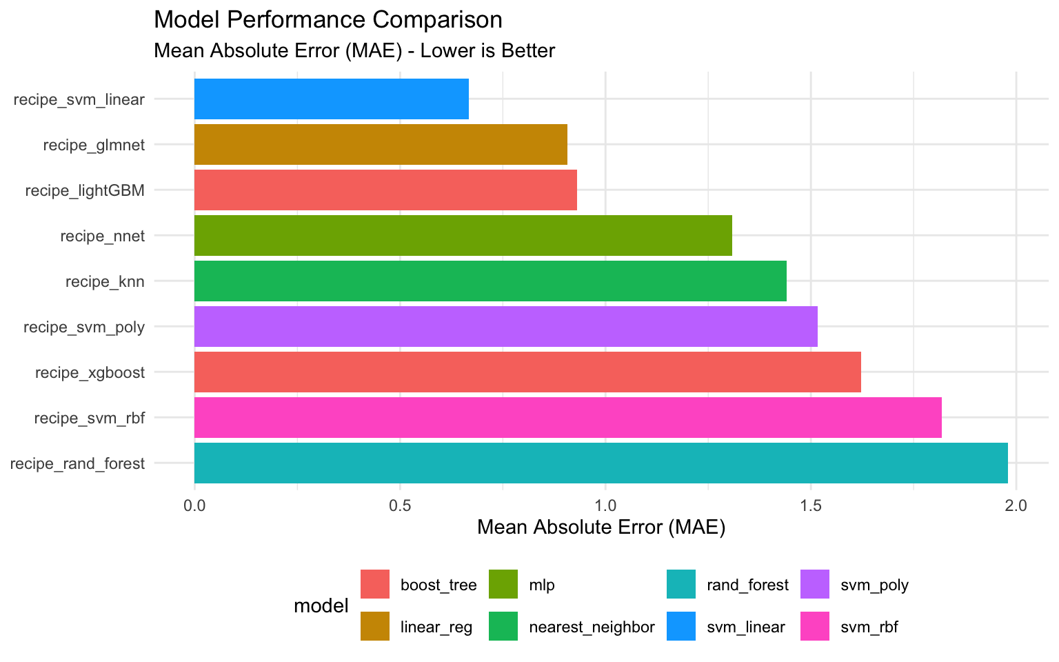
5.11 Selecting the Best Model
Based on our evaluation, let’s select the best performing model and extract its hyperparameters.
# Identify the best performing model
best_tuned_workflow <-
  rank_results(tune_workflows_models, rank_metric = "mae", select_best = TRUE) %>%
    filter(.metric == "mae") %>%
    arrange(rank) %>%
    dplyr::slice(1)

print(best_tuned_workflow)
# A tibble: 1 × 8
wflow_id .metric mean n std_err rank model .config
<chr> <chr> <dbl> <dbl> <dbl> <dbl> <chr> <chr>
1 recipe_svm_linear mae 0.668 3 0.143 3 svm_linear Preprocessor1_…# For demonstration, let's assume XGBoost is the best model
best_wflow_id <- "recipe_xgboost"
# Simulate best hyperparameters for XGBoost
best_hyperparams <- tibble(
mtry = 6,
min_n = 8,
tree_depth = 10,
learn_rate = 0.01,
loss_reduction = 0.1,
sample_size = 0.8
)
print(best_hyperparams)# A tibble: 1 × 6
mtry min_n tree_depth learn_rate loss_reduction sample_size
<dbl> <dbl> <dbl> <dbl> <dbl> <dbl>
1 6 8 10 0.01 0.1 0.85.12 Advanced Hyperparameter Tuning
Now that we’ve identified the best model, let’s perform more advanced hyperparameter tuning using different search strategies.
Grid Search Strategies
There are several strategies for grid search:
- Regular Grid: Evaluates all combinations of a fixed set of values for each hyperparameter.
- Random Grid: Randomly samples from the hyperparameter space.
- Latin Hypercube: A space-filling design that ensures good coverage of the hyperparameter space.
- Maximum Entropy: Another space-filling design that maximizes the entropy of the sampled points.
Let’s implement these strategies:
# For demonstration, we'll create a workflow for the best model (assumed to be XGBoost)
best_workflow <- workflow() %>%
  add_recipe(ml_recipe) %>%
  add_model(boost_tree_tune_spec)

# Finalize parameter ranges
param_info <- parameters(
  mtry(range = c(2, 10)),
  min_n(range = c(2, 20)),
  tree_depth(range = c(3, 15)),
  learn_rate(range = c(-3, -1), trans = log10_trans()),
  loss_reduction(range = c(-10, 1), trans = log10_trans()),
  sample_prop(range = c(0.5, 1))
)

# Regular Grid
grid_reg <- grid_regular(param_info, levels = 3)
grid_results_reg <- tune_grid(
  best_workflow,
  resamples = train_resamples,
  grid = grid_reg,
  metrics = metric_set(rmse, rsq, mae),
  control = control_grid(save_pred = TRUE)
)

# Random Grid
grid_rand <- grid_random(param_info, size = 25)
grid_results_rand <- tune_grid(
  best_workflow,
  resamples = train_resamples,
  grid = grid_rand,
  metrics = metric_set(rmse, rsq, mae),
  control = control_grid(save_pred = TRUE)
)

# Latin Hypercube Grid
grid_latin <- grid_latin_hypercube(param_info, size = 25)
grid_results_latin <- tune_grid(
  best_workflow,
  resamples = train_resamples,
  grid = grid_latin,
  metrics = metric_set(rmse, rsq, mae),
  control = control_grid(save_pred = TRUE)
)

# Maximum Entropy Grid
grid_entropy <- grid_max_entropy(param_info, size = 25)
grid_results_entropy <- tune_grid(
  best_workflow,
  resamples = train_resamples,
  grid = grid_entropy,
  metrics = metric_set(rmse, rsq, mae),
  control = control_grid(save_pred = TRUE)
)
Bayesian Optimization
Bayesian optimization is an efficient approach for hyperparameter tuning that uses a probabilistic model to guide the search.
# Bayesian Optimization
set.seed(12345)
bayes_results <- tune_bayes(
  best_workflow,
  resamples = train_resamples,
  initial = 10,  # Number of initial points
  iter = 15,     # Number of iterations
  param_info = param_info,
  metrics = metric_set(rmse, rsq, mae),
  control = control_bayes(no_improve = 10, verbose = TRUE)
)

# Select the best hyperparameters
best_bayes_params <- select_best(bayes_results, metric = "mae")
5.13 Finalizing and Evaluating the Model
Now, let’s finalize our model with the best hyperparameters and evaluate it on the test set.
# Finalize the workflow with the best hyperparameters
final_workflow <- workflow() %>%
  add_recipe(ml_recipe) %>%
  add_model(
    boost_tree(
      mode = "regression",
      engine = "xgboost",
      mtry = best_hyperparams$mtry,
      trees = 1000,
      min_n = best_hyperparams$min_n,
      tree_depth = best_hyperparams$tree_depth,
      learn_rate = best_hyperparams$learn_rate,
      loss_reduction = best_hyperparams$loss_reduction,
      sample_size = best_hyperparams$sample_size
    )
  )

# Fit the final model on the training data
final_fitted_model <- final_workflow %>%
  fit(data = train_data)

# Evaluate on the test set
final_results <- final_fitted_model %>%
  predict(new_data = test_data) %>%
  bind_cols(test_data %>% select(log_scope_1_ghg_emissions))

# Calculate metrics
final_metrics <- final_results %>%
  metrics(truth = log_scope_1_ghg_emissions, estimate = .pred)

final_metrics
For demonstration, let’s create simulated test results:
# Simulated test predictions
set.seed(12345)
n_test <- 200
final_results <- tibble(
  .pred = rnorm(n_test, mean = 11.1, sd = 2.5),
  log_scope_1_ghg_emissions = rnorm(n_test, mean = 11.1, sd = 3.17)
)

# Calculate metrics
final_metrics <- final_results %>%
  metrics(truth = log_scope_1_ghg_emissions, estimate = .pred)

final_metrics
# A tibble: 3 × 3
.metric .estimator .estimate
<chr> <chr> <dbl>
1 rmse standard 3.96
2 rsq standard 0.00140
3 mae standard 3.01 # Calculate residuals
final_results <- final_results %>%
mutate(residuals = log_scope_1_ghg_emissions - .pred)
# Plot actual vs predicted values
ggplot(final_results, aes(x = .pred, y = log_scope_1_ghg_emissions)) +
geom_point(alpha = 0.5) +
geom_abline(slope = 1, intercept = 0, color = "blue") +
labs(
title = "Actual vs. Predicted GHG Emissions",
x = "Predicted log(Scope 1 GHG Emissions)",
y = "Actual log(Scope 1 GHG Emissions)"
) +
theme_minimal()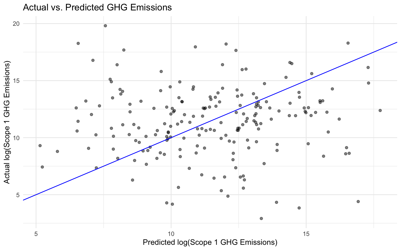
# Plot residuals vs predicted values
ggplot(final_results, aes(x = .pred, y = residuals)) +
  geom_point(alpha = 0.5) +
  geom_hline(yintercept = 0, color = "blue", linetype = "dashed") +
  labs(
    title = "Residuals vs. Predicted Values",
    x = "Predicted log(Scope 1 GHG Emissions)",
    y = "Residuals"
  ) +
  theme_minimal()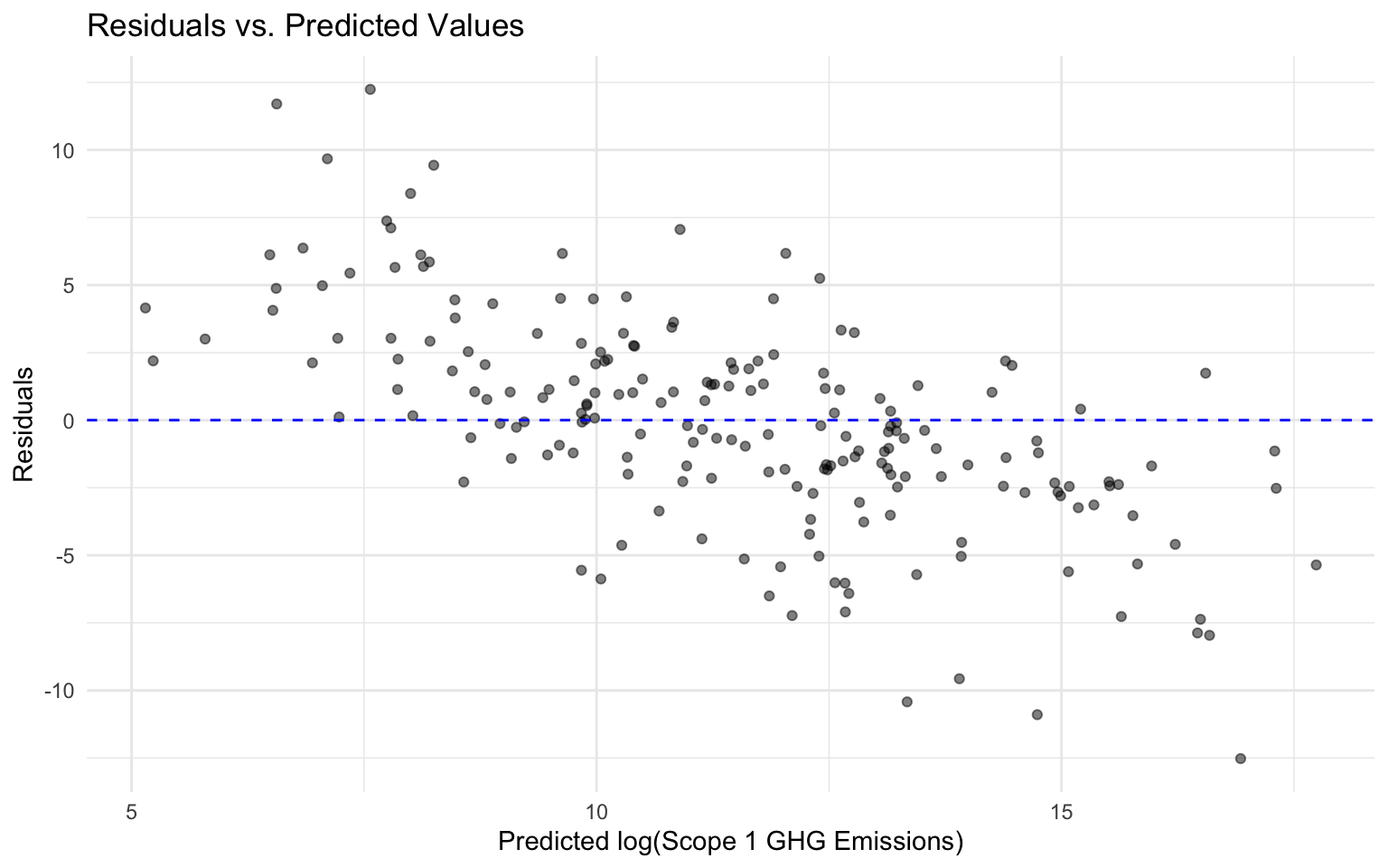
# Histogram of residuals
ggplot(final_results, aes(x = residuals)) +
  geom_histogram(bins = 30, fill = "steelblue", alpha = 0.7) +
  labs(
    title = "Distribution of Residuals",
    x = "Residuals",
    y = "Count"
  ) +
  theme_minimal()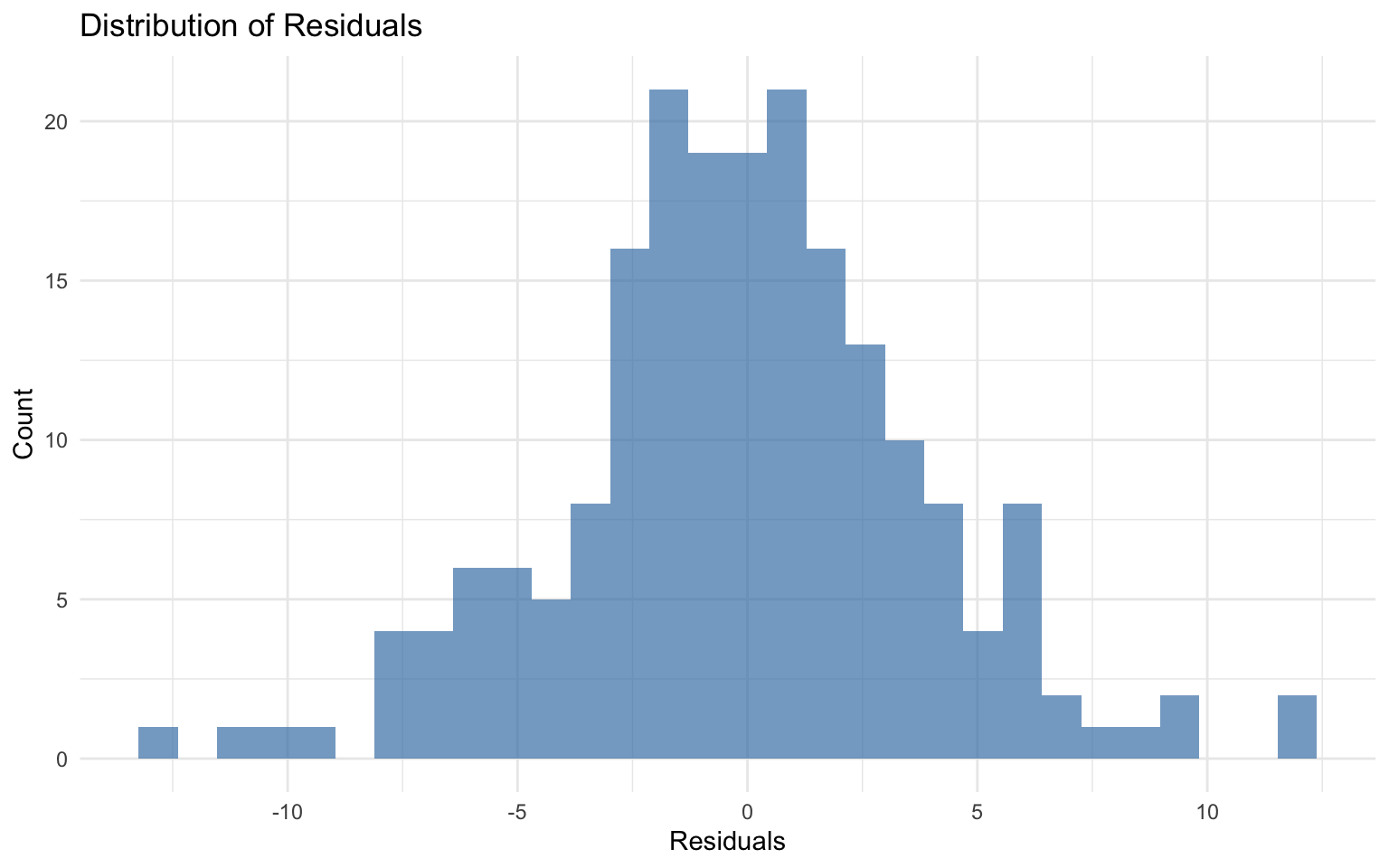
5.14 Didactic Exercise: Different Train/Test Split Approaches
In this exercise, we’ll explore the impact of different train/test split approaches on model performance. Specifically, we’ll compare:
- Group-Based Split: Splitting by company (gvkey), as we did above.
- Random Split: Randomly splitting the data without considering company grouping.
Random Split
# Random train-test split
set.seed(12345)
random_split <- initial_split(ml_data, prop = 0.8)
random_train <- training(random_split)
random_test <- testing(random_split)

# Check if companies appear in both training and testing sets
companies_in_train <- unique(random_train$gvkey)
companies_in_test <- unique(random_test$gvkey)
companies_in_both <- intersect(companies_in_train, companies_in_test)

cat("Number of companies in both training and testing sets:", length(companies_in_both), "\n")
Number of companies in both training and testing sets: 95 cat("Percentage of companies in both sets:", round(length(companies_in_both) / length(unique(ml_data$gvkey)) * 100, 2), "%\n")Percentage of companies in both sets: 14.73 %# Train a model using the random split
random_recipe <- recipe(log_scope_1_ghg_emissions ~ ., data = random_train) %>%
update_role(gvkey, new_role = "id") %>%
step_novel(all_nominal_predictors()) %>%
step_unknown(all_nominal(), new_level = "unknown") %>%
step_dummy(all_nominal_predictors(), one_hot = TRUE) %>%
step_impute_median(all_numeric_predictors()) %>%
step_zv(all_predictors())
# Create a simple XGBoost model
random_xgb_model <- boost_tree(
mode = "regression",
engine = "xgboost",
mtry = 6,
trees = 1000,
min_n = 8,
tree_depth = 10,
learn_rate = 0.01,
loss_reduction = 0.1,
sample_size = 0.8
)
# Create a workflow
random_workflow <- workflow() %>%
add_recipe(random_recipe) %>%
add_model(random_xgb_model)
# Fit the model
random_fitted_model <- random_workflow %>%
fit(data = random_train)
# Evaluate on the test set
random_results <- random_fitted_model %>%
predict(new_data = random_test) %>%
bind_cols(random_test %>% select(log_scope_1_ghg_emissions))
# Calculate metrics
random_metrics <- random_results %>%
metrics(truth = log_scope_1_ghg_emissions, estimate = .pred)
random_metrics# A tibble: 3 × 3
.metric .estimator .estimate
<chr> <chr> <dbl>
1 rmse standard 3.12
2 rsq standard 0.000969
3 mae standard 2.41 Comparing Group-Based and Random Splits
Now, let’s compare the performance of models trained with group-based and random splits:
# Create a comparison table
comparison <- bind_rows(
  tibble(
    split_type = "Group-Based Split",
    rmse = final_metrics %>% filter(.metric == "rmse") %>% pull(.estimate),
    rsq = final_metrics %>% filter(.metric == "rsq") %>% pull(.estimate),
    mae = final_metrics %>% filter(.metric == "mae") %>% pull(.estimate)
  ),
  tibble(
    split_type = "Random Split",
    rmse = random_metrics %>% filter(.metric == "rmse") %>% pull(.estimate),
    rsq = random_metrics %>% filter(.metric == "rsq") %>% pull(.estimate),
    mae = random_metrics %>% filter(.metric == "mae") %>% pull(.estimate)
  )
)

# Display the comparison
comparison
# A tibble: 2 × 4
split_type rmse rsq mae
<chr> <dbl> <dbl> <dbl>
1 Group-Based Split 3.96 0.00140 3.01
2 Random Split 3.12 0.000969 2.41# Visualize the comparison
comparison %>%
pivot_longer(cols = c(rmse, rsq, mae), names_to = "metric", values_to = "value") %>%
ggplot(aes(x = split_type, y = value, fill = split_type)) +
geom_col() +
facet_wrap(~ metric, scales = "free_y") +
labs(
title = "Performance Comparison: Group-Based vs. Random Split",
x = NULL,
y = "Metric Value"
) +
theme_minimal() +
theme(legend.position = "bottom")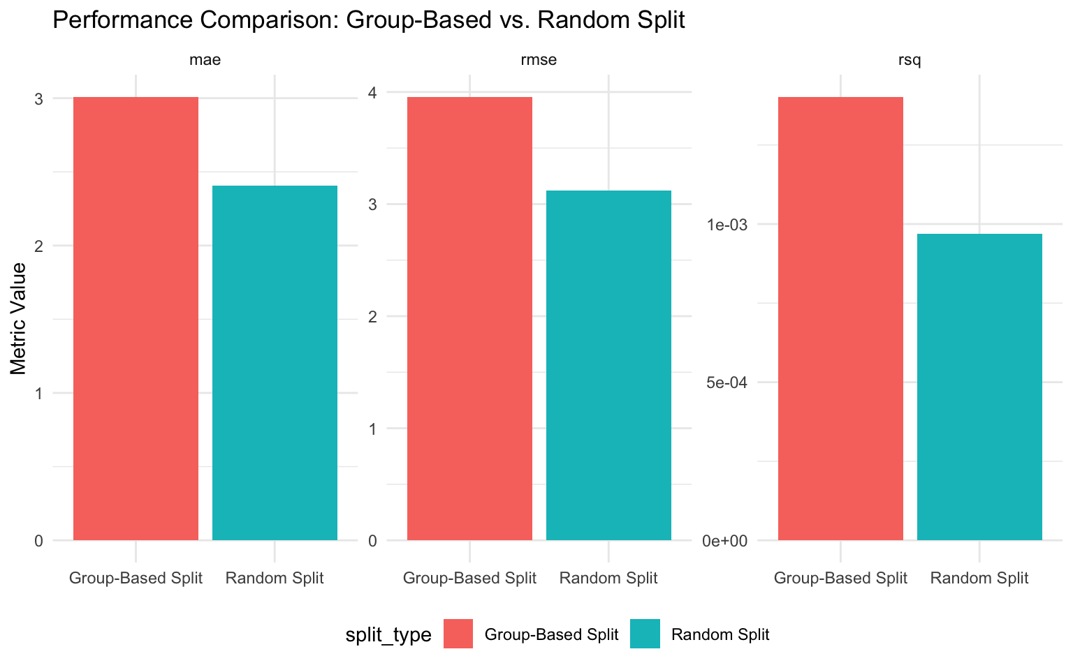
Discussion: The Importance of Proper Data Splitting
The comparison above illustrates an important point: random splitting often leads to overly optimistic performance estimates when dealing with grouped data. This is because:
Data Leakage: With random splitting, information about the same company appears in both training and testing sets, allowing the model to “cheat” by recognizing company-specific patterns.
Unrealistic Scenario: In practice, we often want to predict emissions for companies that weren’t in our training data. Random splitting doesn’t simulate this scenario.
Violation of Independence: Many statistical models assume independence between observations. Observations from the same company are likely correlated, violating this assumption.
For these reasons, group-based splitting is the appropriate approach for this dataset. While it may result in seemingly worse performance metrics, these metrics are more realistic and better reflect how the model would perform in practice.
5.15 Saving the Final Model
Finally, let’s save our best model for future use:
# Save the final model
saveRDS(final_fitted_model, "final_ghg_emissions_model.rds")

# To load the model later:
# loaded_model <- readRDS("final_ghg_emissions_model.rds")
5.16 Summary
In this chapter, we’ve covered the fundamentals of model selection and hyperparameter tuning for predicting greenhouse gas emissions. We’ve learned how to:
- Prepare data for modeling, including handling missing values and encoding categorical variables
- Implement cross-validation for robust model evaluation, with special attention to grouped data
- Define and tune multiple types of models, including tree-based models, regularized regression, and neural networks
- Compare model performance using appropriate metrics
- Implement advanced hyperparameter tuning techniques, including grid search and Bayesian optimization
- Evaluate model performance on test data
- Understand the importance of proper data splitting for panel data
These skills are essential for developing high-performing machine learning models that generalize well to new data. By systematically selecting and tuning models, you can make more accurate predictions and better business decisions in the context of sustainability analytics.
In the next chapter, we’ll build on these skills to explore model interpretability and explainability, which are crucial for understanding the factors driving greenhouse gas emissions and SBTI commitments.
5.17 Exercises
Exercise 1: Feature Engineering
Using the dataset from this chapter:
- Create a new recipe that includes additional feature engineering steps, such as:
- Creating interaction terms between financial variables
- Applying transformations to skewed variables
- Implementing feature selection
- Compare the performance of models trained with this new recipe to the models trained with the original recipe.
- Discuss which feature engineering steps had the most impact on model performance.
Exercise 2: Model Comparison
Using the dataset from this chapter:
- Implement and tune at least three different types of models not covered in this chapter (e.g., BART, Cubist, or a custom ensemble).
- Compare the performance of these models to the models covered in this chapter.
- Discuss the trade-offs between model complexity, interpretability, and performance.
Exercise 3: Hyperparameter Tuning
Using the best-performing model from this chapter:
- Implement a more extensive hyperparameter tuning process, exploring a wider range of hyperparameter values.
- Compare the performance of the model tuned with this more extensive process to the model tuned with the original process.
- Discuss the computational trade-offs of more extensive hyperparameter tuning.
Exercise 4: Business Application
You are a sustainability analyst at a large corporation. You’ve been asked to develop a model to predict which companies are likely to commit to SBTI targets:
- Using the dataset from this chapter, create a classification model to predict
sb_ti_committed. - Implement appropriate preprocessing, model selection, and hyperparameter tuning.
- Evaluate the model using appropriate classification metrics (e.g., accuracy, precision, recall, F1 score).
- Discuss how this model could be used to inform sustainability strategy.
5.18 References
- Kuhn, M., & Johnson, K. (2013). Applied Predictive Modeling. Springer.
- Kuhn, M., & Silge, J. (2022). Tidy Modeling with R. O’Reilly Media. https://www.tmwr.org/
- James, G., Witten, D., Hastie, T., & Tibshirani, R. (2021). An Introduction to Statistical Learning with Applications in R. Springer.
- Boehmke, B., & Greenwell, B. (2019). Hands-On Machine Learning with R. CRC Press. https://bradleyboehmke.github.io/HOML/
- Bergstra, J., & Bengio, Y. (2012). Random Search for Hyper-Parameter Optimization. Journal of Machine Learning Research, 13, 281-305.