# Install required packages if not already installed
if (!require("tidyverse")) install.packages("tidyverse")
if (!require("tidymodels")) install.packages("tidymodels")
if (!require("rpart")) install.packages("rpart")
if (!require("rpart.plot")) install.packages("rpart.plot")
if (!require("ranger")) install.packages("ranger")
if (!require("vip")) install.packages("vip")
if (!require("pROC")) install.packages("pROC")
if (!require("ROSE")) install.packages("ROSE")
if (!require("themis")) install.packages("themis")4 🔍 Predictive Modeling II: Probabilistic & 🌳 Tree-Based Classification
4.1 Learning Objectives
By the end of this chapter, you will be able to:
- Understand the principles of classification for business applications
- Implement logistic regression models for binary classification
- Apply tree-based classification algorithms including decision trees and random forests
- Evaluate classification model performance using appropriate metrics
- Interpret classification results in business contexts
- Handle class imbalance in classification problems
- Compare and select models based on business requirements
- Visualize classification results for business presentations
4.2 Prerequisites
For this chapter, you’ll need:
- R and RStudio installed on your computer
- Understanding of data manipulation with dplyr (covered in Chapter 1)
- Basic knowledge of data visualization with ggplot2 (covered in Chapter 2)
- Familiarity with regression analysis (covered in Chapter 3)
- The following R packages installed:
# Load required packages
library(tidyverse)      # For data manipulation and visualization
library(tidymodels)     # For modeling framework
library(rpart)          # For decision trees
library(rpart.plot)     # For plotting decision trees
library(ranger)         # For random forests
library(vip)            # For variable importance plots
library(pROC)           # For ROC curves
library(ROSE)           # For handling class imbalance
library(themis)         # For handling class imbalance in recipes
4.3 Introduction to Classification
Classification is a supervised learning technique used to predict categorical outcomes. It’s one of the most widely used techniques in business analytics for predicting customer behavior, risk assessment, and decision-making.
Why Classification in Business?
Classification models are valuable in business for several reasons:
- Customer Segmentation: Identifying customer groups for targeted marketing
- Churn Prediction: Predicting which customers are likely to leave
- Credit Scoring: Assessing creditworthiness and default risk
- Fraud Detection: Identifying fraudulent transactions
- Product Recommendation: Recommending products based on customer preferences
- Quality Control: Detecting defective products
Types of Classification Models
There are several types of classification models, each with its own strengths and weaknesses:
- Logistic Regression: A probabilistic approach for binary classification
- Decision Trees: Rule-based models with a tree-like structure
- Random Forests: Ensemble of decision trees for improved accuracy
- Support Vector Machines: Models that find the optimal boundary between classes
- Naive Bayes: Probabilistic classifiers based on Bayes’ theorem
- Neural Networks: Deep learning models for complex patterns
In this chapter, we’ll focus on logistic regression and tree-based methods, which are widely used in business applications.
4.4 Binary Classification with Logistic Regression
Logistic regression is a statistical method for binary classification that models the probability of an observation belonging to a particular category.
The Logistic Regression Model
The logistic regression model is:
\[P(Y = 1) = \frac{1}{1 + e^{-(\beta_0 + \beta_1 X_1 + \beta_2 X_2 + \ldots + \beta_p X_p)}}\]
Where: - \(P(Y = 1)\) is the probability of the positive class - \(X_1, X_2, \ldots, X_p\) are the independent variables - \(\beta_0, \beta_1, \beta_2, \ldots, \beta_p\) are the coefficients
The logit transformation converts this to a linear model:
\[\log\left(\frac{P(Y = 1)}{1 - P(Y = 1)}\right) = \beta_0 + \beta_1 X_1 + \beta_2 X_2 + \ldots + \beta_p X_p\]
Implementing Logistic Regression in R
Let’s start with a simple example using the Default dataset from the ISLR package, which contains information about credit card default:
# Load the ISLR package for the Default dataset
if (!require("ISLR")) install.packages("ISLR")
Loading required package: ISLRWarning: package 'ISLR' was built under R version 4.4.1library(ISLR)
# Explore the data
glimpse(Default)Rows: 10,000
Columns: 4
$ default <fct> No, No, No, No, No, No, No, No, No, No, No, No, No, No, No, No…
$ student <fct> No, Yes, No, No, No, Yes, No, Yes, No, No, Yes, Yes, No, No, N…
$ balance <dbl> 729.5265, 817.1804, 1073.5492, 529.2506, 785.6559, 919.5885, 8…
$ income <dbl> 44361.625, 12106.135, 31767.139, 35704.494, 38463.496, 7491.55…# Convert to a tibble for better printing
default_data <- as_tibble(Default)
# Check the class distribution
default_data %>%
count(default) %>%
mutate(pct = n / sum(n) * 100)# A tibble: 2 × 3
default n pct
<fct> <int> <dbl>
1 No 9667 96.7
2 Yes 333 3.33Let’s visualize the relations between default status and some predictors:
# Visualize the relation between balance and default
ggplot(default_data, aes(x = balance, fill = default)) +
  geom_histogram(position = "fill", bins = 30) +
  labs(
    title = "Probability of Default by Balance",
    x = "Balance",
    y = "Proportion",
    fill = "Default"
  ) +
  theme_minimal()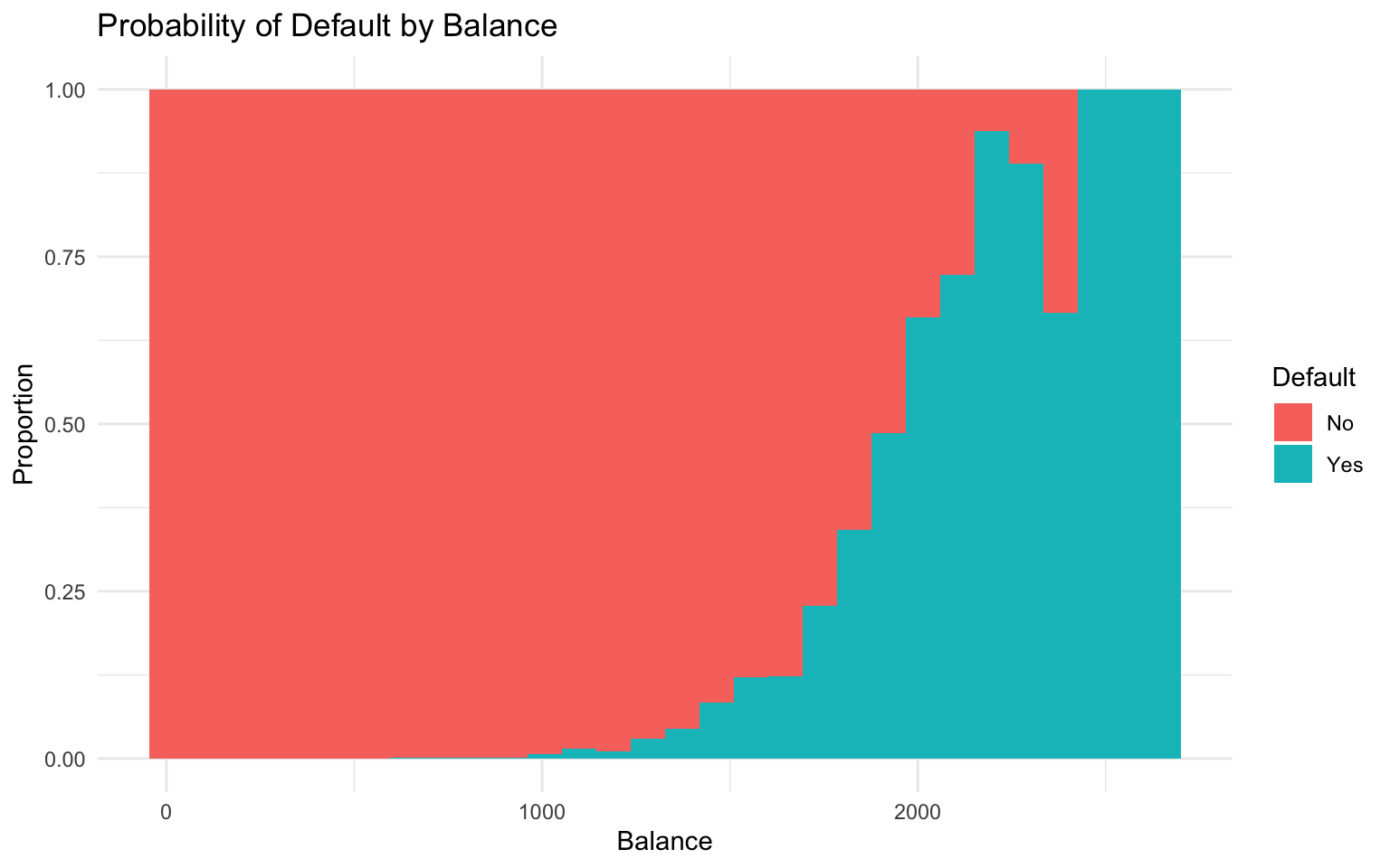
# Visualize the relation between income and default
ggplot(default_data, aes(x = income, fill = default)) +
  geom_histogram(position = "fill", bins = 30) +
  labs(
    title = "Probability of Default by Income",
    x = "Income",
    y = "Proportion",
    fill = "Default"
  ) +
  theme_minimal()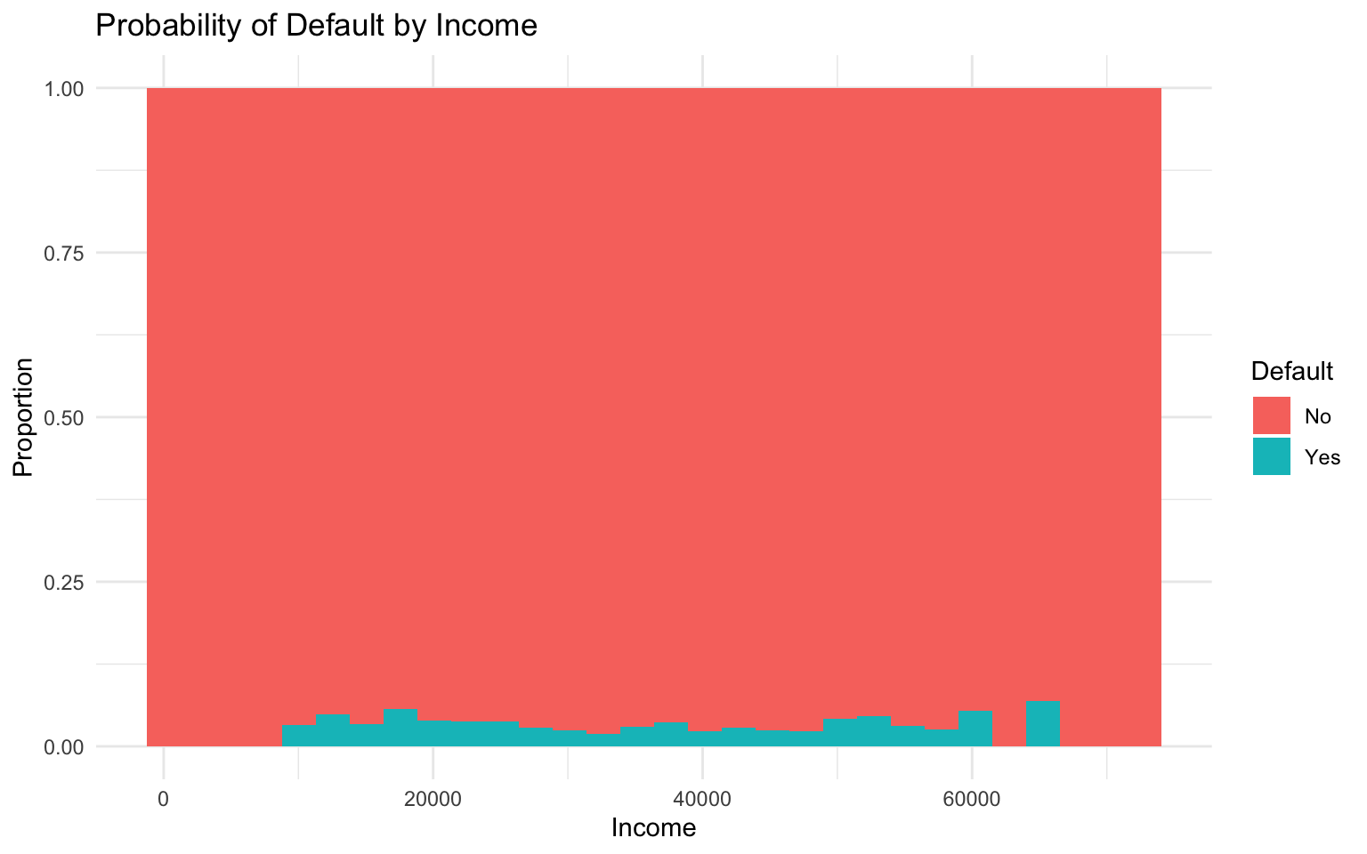
# Visualize the relation between student status and default
ggplot(default_data, aes(x = student, fill = default)) +
  geom_bar(position = "fill") +
  labs(
    title = "Probability of Default by Student Status",
    x = "Student",
    y = "Proportion",
    fill = "Default"
  ) +
  theme_minimal()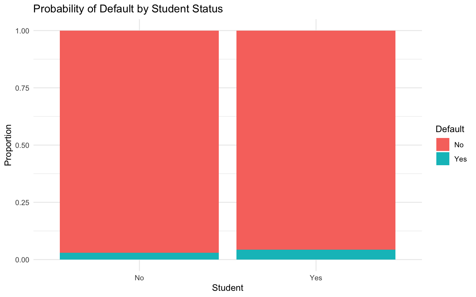
Now, let’s fit a logistic regression model:
# Split the data into training and testing sets
set.seed(123)
default_split <- initial_split(default_data, prop = 0.75, strata = default)
default_train <- training(default_split)
default_test <- testing(default_split)

# Fit a logistic regression model
logistic_model <- glm(default ~ balance + income + student,
                      data = default_train,
                      family = "binomial")

# View the model summary
summary(logistic_model)
Call:
glm(formula = default ~ balance + income + student, family = "binomial",
    data = default_train)

Coefficients:
              Estimate Std. Error z value Pr(>|z|)
(Intercept) -1.088e+01  5.748e-01 -18.922   <2e-16 ***
balance      5.780e-03  2.701e-04  21.398   <2e-16 ***
income       5.678e-07  9.613e-06   0.059    0.953
studentYes  -7.005e-01  2.754e-01  -2.544    0.011 *
---
Signif. codes:  0 '***' 0.001 '**' 0.01 '*' 0.05 '.' 0.1 ' ' 1

(Dispersion parameter for binomial family taken to be 1)

    Null deviance: 2158.4  on 7499  degrees of freedom
Residual deviance: 1138.7  on 7496  degrees of freedom
AIC: 1146.7

Number of Fisher Scoring iterations: 8
Interpreting Logistic Regression Results
The coefficients in logistic regression represent the change in the log odds of the positive class for a one-unit increase in the predictor, holding other predictors constant.
To make the interpretation more intuitive, we can convert the coefficients to odds ratios by exponentiating them:
# Convert coefficients to odds ratios
odds_ratios <- exp(coef(logistic_model))
odds_ratios
(Intercept) balance income studentYes
1.891114e-05 1.005797e+00 1.000001e+00 4.963453e-01 For example, the odds ratio for balance is 1.0058, meaning that for each additional dollar in balance, the odds of default increase by a factor of 1.0058, holding other variables constant.
For categorical variables like student, the odds ratio represents the odds of default for students compared to non-students, holding other variables constant.
Making Predictions with Logistic Regression
We can use the model to make predictions on the test set:
# Make predictions on the test set
default_pred <- default_test %>%
  mutate(
    default_prob = predict(logistic_model, newdata = default_test, type = "response"),
    default_pred = ifelse(default_prob > 0.5, "Yes", "No"),
    default_pred = factor(default_pred, levels = c("No", "Yes"))
  )

# View the first few predictions
default_pred %>%
  select(default, default_prob, default_pred) %>%
  head(10)
# A tibble: 10 × 3
default default_prob default_pred
<fct> <dbl> <fct>
1 No 0.00191 No
2 No 0.000325 No
3 No 0.00864 No
4 No 0.000786 No
5 No 0.0796 No
6 No 0.00380 No
7 No 0.0345 No
8 No 0.00106 No
9 No 0.000147 No
10 No 0.000843 No Evaluating Logistic Regression Performance
To evaluate the performance of our logistic regression model, we can use various metrics:
# Create a confusion matrix
conf_mat <- conf_mat(default_pred, truth = default, estimate = default_pred)
conf_mat
Truth
Prediction No Yes
No 2405 65
Yes 7 23# Calculate accuracy, precision, recall, and F1 score
metrics <- metric_set(accuracy, precision, recall, f_meas)
metrics(default_pred, truth = default, estimate = default_pred)# A tibble: 4 × 3
.metric .estimator .estimate
<chr> <chr> <dbl>
1 accuracy binary 0.971
2 precision binary 0.974
3 recall binary 0.997
4 f_meas binary 0.985We can also create an ROC curve to visualize the trade-off between sensitivity and specificity:
# Create an ROC curve using pROC package for better curve properties
roc_obj <- roc(default_pred$default, default_pred$default_prob)
Setting levels: control = No, case = YesSetting direction: controls < casesauc_value <- round(auc(roc_obj), 3)
# Plot the ROC curve
ggroc(roc_obj) +
geom_abline(slope = 1, intercept = 1, linetype = "dashed", color = "gray") +
labs(
title = "ROC Curve for Logistic Regression Model",
subtitle = paste("AUC =", auc_value)
) +
theme_minimal()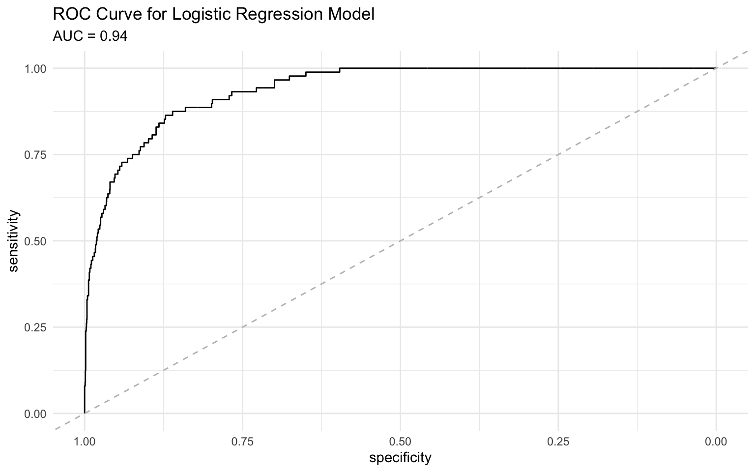
Visualizing Logistic Regression Results
We can visualize the relation between predictors and the predicted probability of default:
# Create a grid of balance values
balance_grid <- tibble(
  balance = seq(min(default_data$balance), max(default_data$balance), length.out = 100),
  income = mean(default_data$income),
  student = "No"
)

# Make predictions on the grid
balance_grid <- balance_grid %>%
  mutate(default_prob = predict(logistic_model, newdata = balance_grid, type = "response"))

# Plot the relation
ggplot(balance_grid, aes(x = balance, y = default_prob)) +
  geom_line() +
  geom_hline(yintercept = 0.5, linetype = "dashed", color = "red") +
  labs(
    title = "Probability of Default by Balance",
    x = "Balance",
    y = "Probability of Default"
  ) +
  theme_minimal()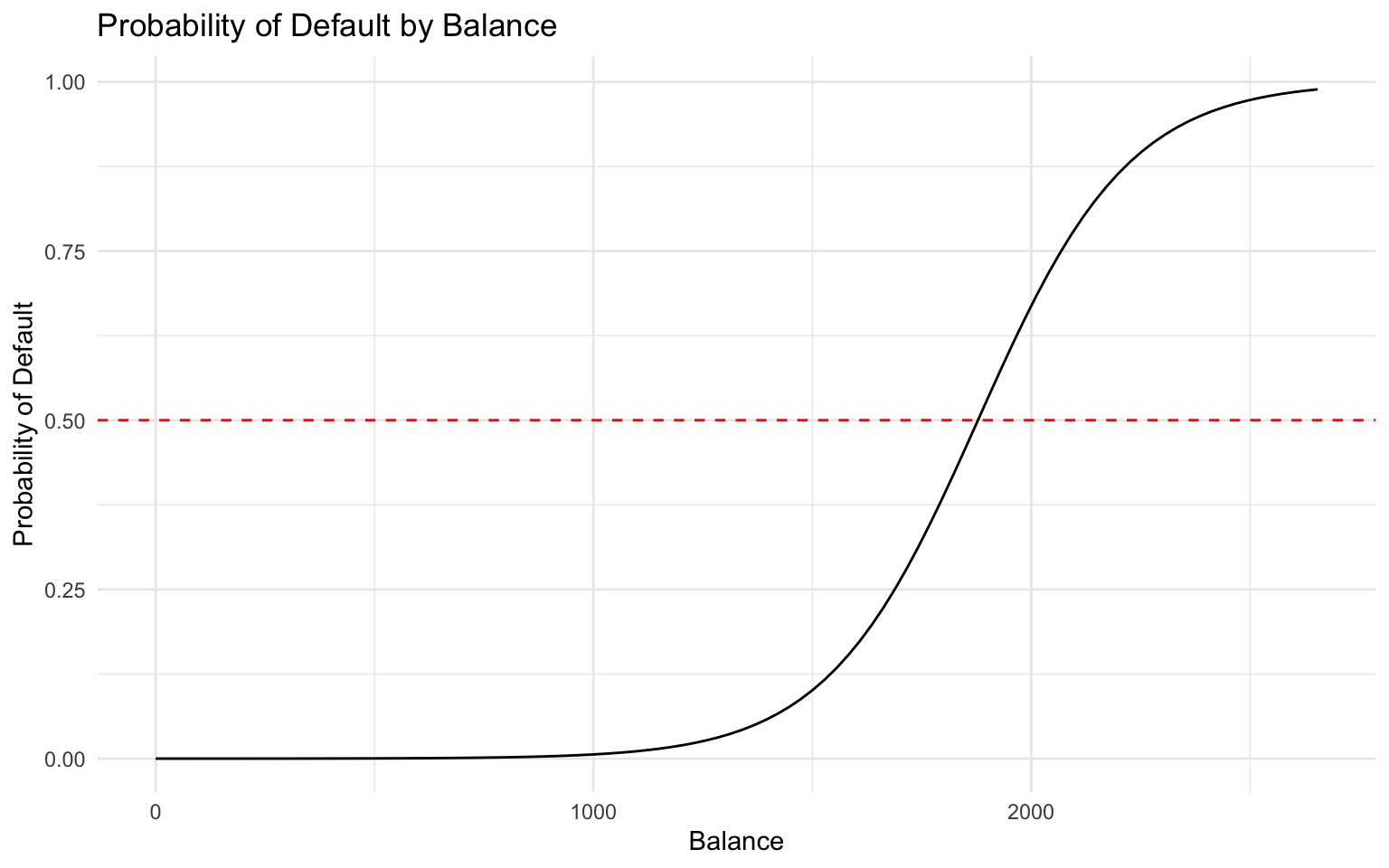
4.5 Decision Trees
Decision trees are rule-based models that recursively split the data based on the values of the predictors to create homogeneous groups.
How Decision Trees Work
Decision trees work by:
- Selecting the best feature to split the data
- Creating child nodes based on the split
- Recursively repeating the process for each child node
- Stopping when a stopping criterion is met (e.g., maximum depth, minimum samples per leaf)
The best split is determined by measures like Gini impurity or information gain, which quantify the homogeneity of the resulting nodes.
Implementing Decision Trees in R
Let’s implement a decision tree for the credit default data:
# Fit a decision tree model
tree_model <- rpart(default ~ balance + income + student,
                   data = default_train,
                   method = "class",
                   control = rpart.control(cp = 0.01))

# Plot the decision tree
rpart.plot(tree_model, extra = 101, box.palette = "RdBu", shadow.col = "gray", nn = TRUE)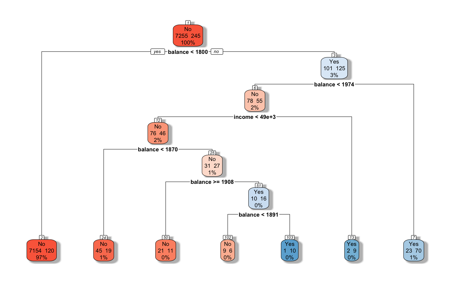
Interpreting Decision Trees
Decision trees are highly interpretable. Each node shows:
- The predicted class
- The probability of the positive class
- The percentage of observations in the node
The splits show the rules used to segment the data. For example, the first split might be “balance < 1000”, meaning that customers with a balance less than $1,000 go to the left branch, and those with a balance of $1,000 or more go to the right branch.
Making Predictions with Decision Trees
We can use the decision tree to make predictions on the test set:
# Make predictions on the test set
tree_pred <- default_test %>%
  mutate(
    default_prob = predict(tree_model, newdata = default_test, type = "prob")[, 2],
    default_pred = predict(tree_model, newdata = default_test, type = "class")
  )

# View the first few predictions
tree_pred %>%
  select(default, default_prob, default_pred) %>%
  head(10)
# A tibble: 10 × 3
default default_prob default_pred
<fct> <dbl> <fct>
1 No 0.0165 No
2 No 0.0165 No
3 No 0.0165 No
4 No 0.0165 No
5 No 0.0165 No
6 No 0.0165 No
7 No 0.0165 No
8 No 0.0165 No
9 No 0.0165 No
10 No 0.0165 No Evaluating Decision Tree Performance
Let’s evaluate the performance of our decision tree model:
# Create a confusion matrix
conf_mat(tree_pred, truth = default, estimate = default_pred)
Truth
Prediction No Yes
No 2405 63
Yes 7 25# Calculate accuracy, precision, recall, and F1 score
metrics(tree_pred, truth = default, estimate = default_pred)# A tibble: 4 × 3
.metric .estimator .estimate
<chr> <chr> <dbl>
1 accuracy binary 0.972
2 precision binary 0.974
3 recall binary 0.997
4 f_meas binary 0.986# Create an ROC curve using pROC package for better curve properties
roc_obj <- roc(tree_pred$default, tree_pred$default_prob)Setting levels: control = No, case = YesSetting direction: controls < casesauc_value <- round(auc(roc_obj), 3)
# Plot the ROC curve
ggroc(roc_obj) +
geom_abline(slope = 1, intercept = 1, linetype = "dashed", color = "gray") +
labs(
title = "ROC Curve for Decision Tree Model",
subtitle = paste("AUC =", auc_value)
) +
theme_minimal()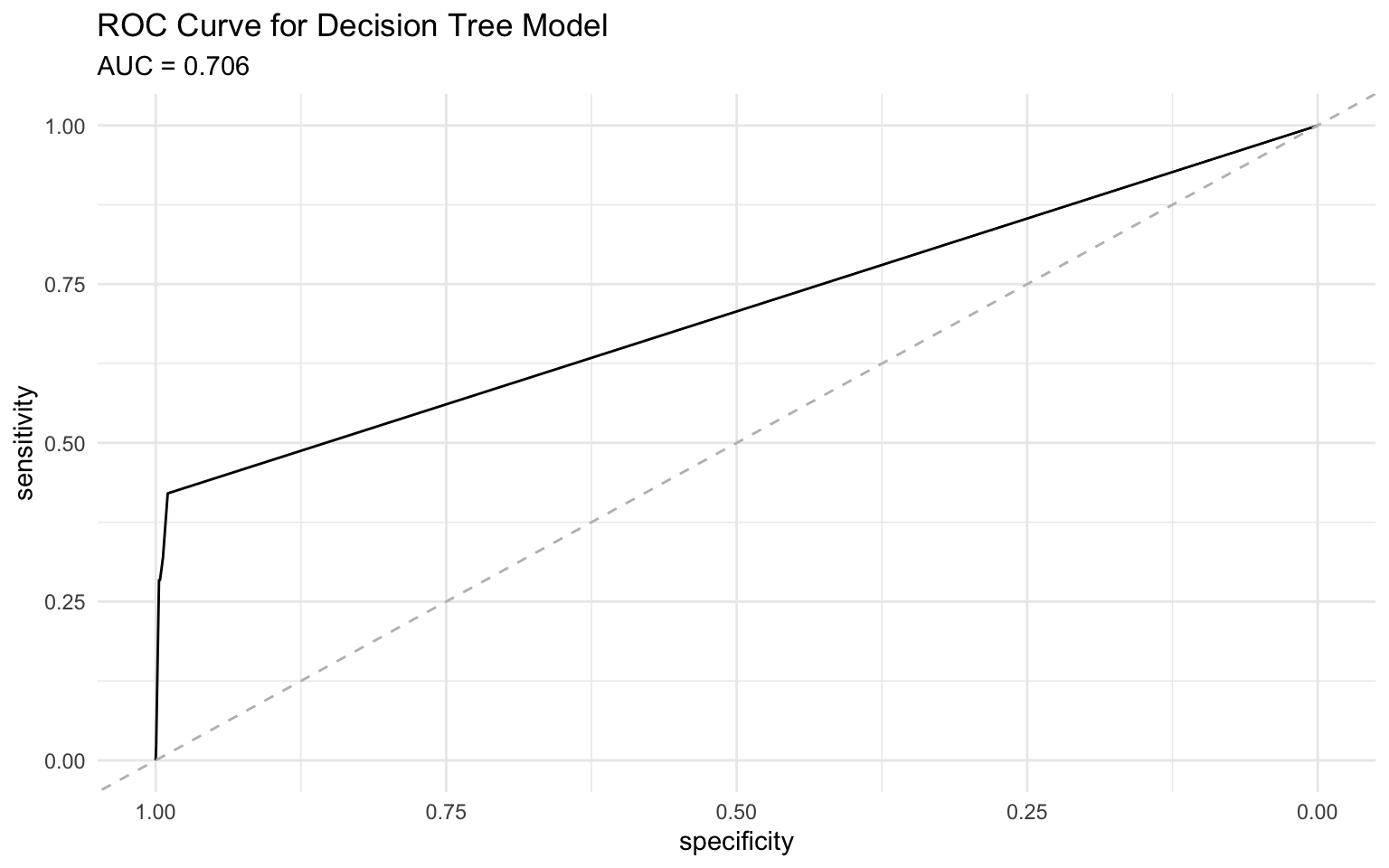
Pruning Decision Trees
Decision trees can be prone to overfitting, where they capture noise in the training data rather than the underlying pattern. Pruning is a technique to reduce overfitting by removing branches that do not significantly improve the model’s performance.
# Plot the complexity parameter table
plotcp(tree_model)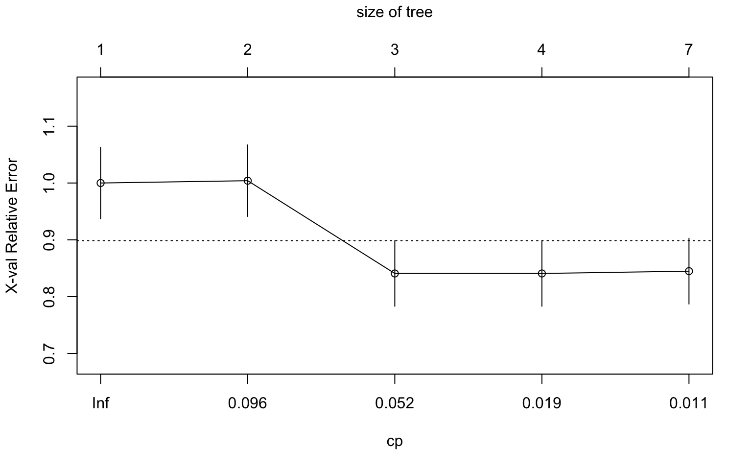
# Print the complexity parameter table
printcp(tree_model)
Classification tree:
rpart(formula = default ~ balance + income + student, data = default_train,
    method = "class", control = rpart.control(cp = 0.01))

Variables actually used in tree construction:
[1] balance income

Root node error: 245/7500 = 0.032667

n= 7500

        CP nsplit rel error  xerror     xstd
1 0.097959      0   1.00000 1.00000 0.062835
2 0.093878      1   0.90204 1.00408 0.062959
3 0.028571      2   0.80816 0.84082 0.057772
4 0.012245      3   0.77959 0.84082 0.057772
5 0.010000      6   0.74286 0.84490 0.057908
# Prune the tree
pruned_tree <- prune(tree_model, cp = 0.02)
# Plot the pruned tree
rpart.plot(pruned_tree, extra = 101, box.palette = "RdBu", shadow.col = "gray", nn = TRUE)
4.6 Random Forests
Random forests are an ensemble learning method that combines multiple decision trees to improve prediction accuracy and reduce overfitting.
How Random Forests Work
Random forests work by:
- Creating multiple decision trees using bootstrap samples of the data
- Randomly selecting a subset of features for each split
- Aggregating the predictions of all trees (majority vote for classification)
This process, known as bagging (bootstrap aggregating) with random feature selection, helps to reduce variance and improve generalization.
Implementing Random Forests in R
Let’s implement a random forest for the credit default data using the ranger package:
# Fit a random forest model
rf_model <- ranger(
  formula = default ~ balance + income + student,
  data = default_train,
  num.trees = 500,
  mtry = 2,
  importance = "impurity",
  probability = TRUE
)

# View the model
rf_model
Ranger result
Call:
ranger(formula = default ~ balance + income + student, data = default_train, num.trees = 500, mtry = 2, importance = "impurity", probability = TRUE)
Type: Probability estimation
Number of trees: 500
Sample size: 7500
Number of independent variables: 3
Mtry: 2
Target node size: 10
Variable importance mode: impurity
Splitrule: gini
OOB prediction error (Brier s.): 0.02379122 Variable Importance in Random Forests
One advantage of random forests is that they provide a measure of variable importance, which indicates how much each feature contributes to the model’s predictive power:
# Extract variable importance
var_importance <- tibble(
  variable = names(importance(rf_model)),
  importance = importance(rf_model)
)

# Plot variable importance
ggplot(var_importance, aes(x = reorder(variable, importance), y = importance)) +
  geom_col() +
  coord_flip() +
  labs(
    title = "Variable Importance in Random Forest Model",
    x = NULL,
    y = "Importance"
  ) +
  theme_minimal()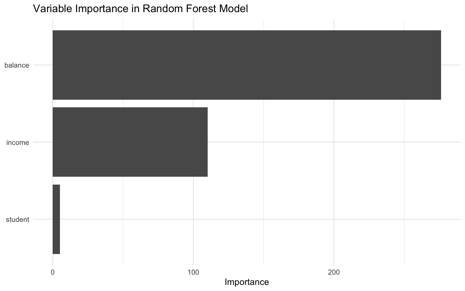
Making Predictions with Random Forests
We can use the random forest to make predictions on the test set:
# Make predictions on the test set
rf_pred <- default_test %>%
  mutate(
    default_prob = predict(rf_model, data = default_test)$predictions[, 2],
    default_pred = ifelse(default_prob > 0.5, "Yes", "No"),
    default_pred = factor(default_pred, levels = c("No", "Yes"))
  )

# View the first few predictions
rf_pred %>%
  select(default, default_prob, default_pred) %>%
  head(10)
# A tibble: 10 × 3
default default_prob default_pred
<fct> <dbl> <fct>
1 No 0 No
2 No 0 No
3 No 0.000222 No
4 No 0 No
5 No 0.00531 No
6 No 0 No
7 No 0.140 No
8 No 0 No
9 No 0 No
10 No 0.01 No Evaluating Random Forest Performance
Let’s evaluate the performance of our random forest model:
# Create a confusion matrix
conf_mat(rf_pred, truth = default, estimate = default_pred)
Truth
Prediction No Yes
No 2399 65
Yes 13 23# Calculate accuracy, precision, recall, and F1 score
metrics(rf_pred, truth = default, estimate = default_pred)# A tibble: 4 × 3
.metric .estimator .estimate
<chr> <chr> <dbl>
1 accuracy binary 0.969
2 precision binary 0.974
3 recall binary 0.995
4 f_meas binary 0.984# Create an ROC curve using pROC package for better curve properties
roc_obj <- roc(rf_pred$default, rf_pred$default_prob)Setting levels: control = No, case = YesSetting direction: controls < casesauc_value <- round(auc(roc_obj), 3)
# Plot the ROC curve
ggroc(roc_obj) +
geom_abline(slope = 1, intercept = 1, linetype = "dashed", color = "gray") +
labs(
title = "ROC Curve for Random Forest Model",
subtitle = paste("AUC =", auc_value)
) +
theme_minimal()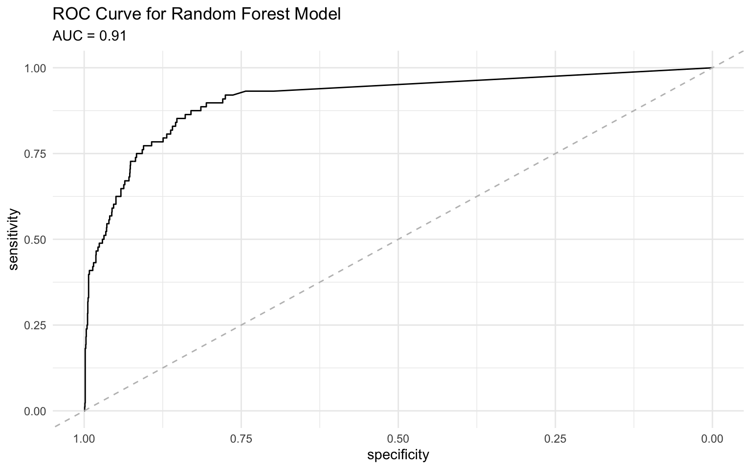
4.7 Comparing Classification Models
Let’s compare the performance of our logistic regression, decision tree, and random forest models:
# Combine predictions from all models
all_preds <- bind_rows(
  default_pred %>%
    select(default, default_prob, default_pred) %>%
    mutate(model = "Logistic Regression"),
  tree_pred %>%
    select(default, default_prob, default_pred) %>%
    mutate(model = "Decision Tree"),
  rf_pred %>%
    select(default, default_prob, default_pred) %>%
    mutate(model = "Random Forest")
)

# Calculate metrics for all models
all_metrics <- all_preds %>%
  group_by(model) %>%
  summarize(
    accuracy = accuracy_vec(default, default_pred),
    precision = precision_vec(default, default_pred),
    recall = recall_vec(default, default_pred),
    f1 = f_meas_vec(default, default_pred),
    auc = roc_auc_vec(default, default_prob)
  )

# View the metrics
all_metrics
# A tibble: 3 × 6
model accuracy precision recall f1 auc
<chr> <dbl> <dbl> <dbl> <dbl> <dbl>
1 Decision Tree 0.972 0.974 0.997 0.986 0.294
2 Logistic Regression 0.971 0.974 0.997 0.985 0.0597
3 Random Forest 0.969 0.974 0.995 0.984 0.0904# Create ROC curves for all models using pROC package
# Create a list to store ROC objects for each model
roc_list <- all_preds %>%
group_by(model) %>%
group_map(~roc(.x$default, .x$default_prob))Setting levels: control = No, case = YesSetting direction: controls < casesSetting levels: control = No, case = YesSetting direction: controls < casesSetting levels: control = No, case = YesSetting direction: controls < cases# Name the ROC objects in the list
names(roc_list) <- unique(all_preds$model)
# Calculate AUC for each model
auc_values <- sapply(roc_list, auc)
auc_labels <- paste0(names(auc_values), " (AUC = ", round(auc_values, 3), ")")
# Plot the ROC curves
ggroc(roc_list) +
geom_abline(slope = 1, intercept = 1, linetype = "dashed", color = "gray") +
scale_color_discrete(labels = auc_labels) +
labs(
title = "ROC Curves for Classification Models",
color = "Model"
) +
theme_minimal()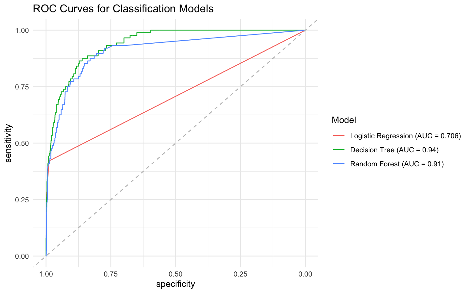
4.8 Handling Class Imbalance
In many business applications, the classes are imbalanced, meaning that one class (usually the one of interest) is much less frequent than the other. This can lead to models that perform poorly on the minority class.
Techniques for Handling Class Imbalance
There are several techniques for handling class imbalance:
- Resampling: Oversampling the minority class or undersampling the majority class
- Synthetic Data Generation: Creating synthetic examples of the minority class (e.g., SMOTE)
- Cost-Sensitive Learning: Assigning higher costs to misclassifying the minority class
- Ensemble Methods: Combining multiple models to improve performance on the minority class
- Threshold Adjustment: Changing the classification threshold to favor the minority class
Let’s demonstrate some of these techniques using the credit default data:
# Check the class distribution
default_train %>%
  count(default) %>%
  mutate(pct = n / sum(n) * 100)
# A tibble: 2 × 3
default n pct
<fct> <int> <dbl>
1 No 7255 96.7
2 Yes 245 3.27Resampling with ROSE
The ROSE (Random Over-Sampling Examples) package provides functions for handling class imbalance:
# Create a balanced dataset using ROSE
balanced_data <- ROSE(default ~ balance + income + student,
                     data = default_train,
                     seed = 123)$data

# Check the class distribution in the balanced data
balanced_data %>%
  count(default) %>%
  mutate(pct = n / sum(n) * 100)
default n pct
1 No 3792 50.56
2 Yes 3708 49.44# Fit a logistic regression model on the balanced data
balanced_model <- glm(default ~ balance + income + student,
data = balanced_data,
family = "binomial")
# Make predictions on the test set
balanced_pred <- default_test %>%
mutate(
default_prob = predict(balanced_model, newdata = default_test, type = "response"),
default_pred = ifelse(default_prob > 0.5, "Yes", "No"),
default_pred = factor(default_pred, levels = c("No", "Yes"))
)
# Evaluate the model
conf_mat(balanced_pred, truth = default, estimate = default_pred) Truth
Prediction No Yes
No 2069 12
Yes 343 76metrics(balanced_pred, truth = default, estimate = default_pred)# A tibble: 4 × 3
.metric .estimator .estimate
<chr> <chr> <dbl>
1 accuracy binary 0.858
2 precision binary 0.994
3 recall binary 0.858
4 f_meas binary 0.921Threshold Adjustment
Another approach is to adjust the classification threshold to favor the minority class:
# Calculate precision and recall at different thresholds
threshold_metrics <- tibble(
  threshold = seq(0.1, 0.9, by = 0.1)
) %>%
  mutate(
    precision = map_dbl(threshold, ~ precision_vec(
      default_pred$default,
      ifelse(default_pred$default_prob > .x, "Yes", "No") %>% factor(levels = c("No", "Yes"))
    )),
    recall = map_dbl(threshold, ~ recall_vec(
      default_pred$default,
      ifelse(default_pred$default_prob > .x, "Yes", "No") %>% factor(levels = c("No", "Yes"))
    )),
    f1 = map_dbl(threshold, ~ f_meas_vec(
      default_pred$default,
      ifelse(default_pred$default_prob > .x, "Yes", "No") %>% factor(levels = c("No", "Yes"))
    ))
  )

# Plot the metrics
threshold_metrics %>%
  pivot_longer(cols = c(precision, recall, f1), names_to = "metric", values_to = "value") %>%
  ggplot(aes(x = threshold, y = value, color = metric)) +
  geom_line() +
  geom_point() +
  labs(
    title = "Precision, Recall, and F1 Score at Different Thresholds",
    x = "Threshold",
    y = "Value",
    color = "Metric"
  ) +
  theme_minimal()
Based on the plot, we can select a threshold that balances precision and recall according to our business requirements.
4.9 Business Case Study: Customer Churn Prediction
Let’s apply classification techniques to a business case study on customer churn prediction.
The Scenario
You’re a data scientist at a telecommunications company. You’ve been asked to develop a model to predict which customers are likely to churn (cancel their service) in the next month. The goal is to identify high-risk customers so that the retention team can take proactive measures to retain them.
The Data
We’ll use a simulated telecom customer churn dataset:
# Create a simulated telecom customer churn dataset
set.seed(123)
n_customers <- 1000

# Generate customer characteristics
telecom_data <- tibble(
  customer_id = 1:n_customers,

  # Demographics
  age = sample(18:80, n_customers, replace = TRUE),
  gender = sample(c("Male", "Female"), n_customers, replace = TRUE),

  # Service information
  tenure_months = sample(1:72, n_customers, replace = TRUE),
  contract = sample(c("Month-to-month", "One year", "Two year"), n_customers, replace = TRUE,
                   prob = c(0.6, 0.2, 0.2)),
  internet_service = sample(c("DSL", "Fiber optic", "No"), n_customers, replace = TRUE),
  online_security = sample(c("Yes", "No", "No internet service"), n_customers, replace = TRUE),
  tech_support = sample(c("Yes", "No", "No internet service"), n_customers, replace = TRUE),

  # Billing information
  monthly_charges = runif(n_customers, min = 20, max = 120),
  total_charges = NA_real_,  # Will calculate based on tenure and monthly charges

  # Customer satisfaction
  satisfaction_score = sample(1:5, n_customers, replace = TRUE, prob = c(0.1, 0.1, 0.2, 0.3, 0.3))
)

# Calculate total charges based on tenure and monthly charges
telecom_data <- telecom_data %>%
  mutate(
    total_charges = tenure_months * monthly_charges * runif(n_customers, min = 0.9, max = 1.1)
  )

# Generate churn based on a logistic model
telecom_data <- telecom_data %>%
  mutate(
    churn_prob = plogis(
      -3 +                                                # Intercept
      -0.03 * tenure_months +                            # Longer tenure, less churn
      ifelse(contract == "Month-to-month", 1.5, 0) +     # Month-to-month more likely to churn
      ifelse(contract == "Two year", -1.5, 0) +          # Two year less likely to churn
      ifelse(internet_service == "Fiber optic", 0.5, 0) + # Fiber customers more likely to churn
      ifelse(tech_support == "Yes", -0.5, 0) +           # Tech support reduces churn
      ifelse(online_security == "Yes", -0.5, 0) +        # Online security reduces churn
      0.01 * monthly_charges +                           # Higher charges, more churn
      -0.3 * satisfaction_score +                        # Higher satisfaction, less churn
      rnorm(n_customers, mean = 0, sd = 0.5)             # Random noise
    ),
    churn = rbinom(n_customers, size = 1, prob = churn_prob)
  ) %>%
  select(-churn_prob) %>%  # Remove the probability column
  mutate(churn = factor(churn, levels = c(0, 1), labels = c("No", "Yes")))  # Convert to factor

# View the data
glimpse(telecom_data)
Rows: 1,000
Columns: 12
$ customer_id <int> 1, 2, 3, 4, 5, 6, 7, 8, 9, 10, 11, 12, 13, 14, 15, …
$ age <int> 48, 32, 68, 31, 20, 59, 67, 71, 60, 54, 69, 31, 71,…
$ gender <chr> "Male", "Male", "Male", "Female", "Female", "Male",…
$ tenure_months <int> 14, 37, 10, 49, 52, 71, 22, 44, 11, 18, 12, 71, 3, …
$ contract <chr> "Month-to-month", "One year", "Month-to-month", "Mo…
$ internet_service <chr> "Fiber optic", "DSL", "No", "Fiber optic", "DSL", "…
$ online_security <chr> "Yes", "No", "No", "No", "Yes", "No", "No", "No", "…
$ tech_support <chr> "No internet service", "Yes", "No internet service"…
$ monthly_charges <dbl> 40.84876, 97.95928, 35.23566, 114.55526, 101.70769,…
$ total_charges <dbl> 580.0644, 3810.2792, 361.0966, 6084.8424, 5308.8745…
$ satisfaction_score <int> 4, 4, 4, 4, 3, 1, 3, 5, 2, 2, 4, 4, 4, 5, 5, 3, 2, …
$ churn <fct> No, No, No, Yes, No, No, No, No, No, No, No, No, No…# Check the class distribution
telecom_data %>%
count(churn) %>%
mutate(pct = n / sum(n) * 100)# A tibble: 2 × 3
churn n pct
<fct> <int> <dbl>
1 No 962 96.2
2 Yes 38 3.8Exploratory Data Analysis
Let’s explore the relations in the data:
# Explore the relation between tenure and churn
ggplot(telecom_data, aes(x = tenure_months, fill = churn)) +
  geom_histogram(position = "fill", bins = 30) +
  labs(
    title = "Churn Rate by Tenure",
    x = "Tenure (Months)",
    y = "Proportion",
    fill = "Churn"
  ) +
  theme_minimal()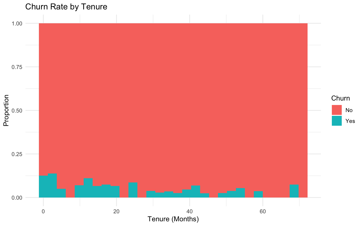
# Explore the relation between contract type and churn
ggplot(telecom_data, aes(x = contract, fill = churn)) +
  geom_bar(position = "fill") +
  labs(
    title = "Churn Rate by Contract Type",
    x = "Contract Type",
    y = "Proportion",
    fill = "Churn"
  ) +
  theme_minimal()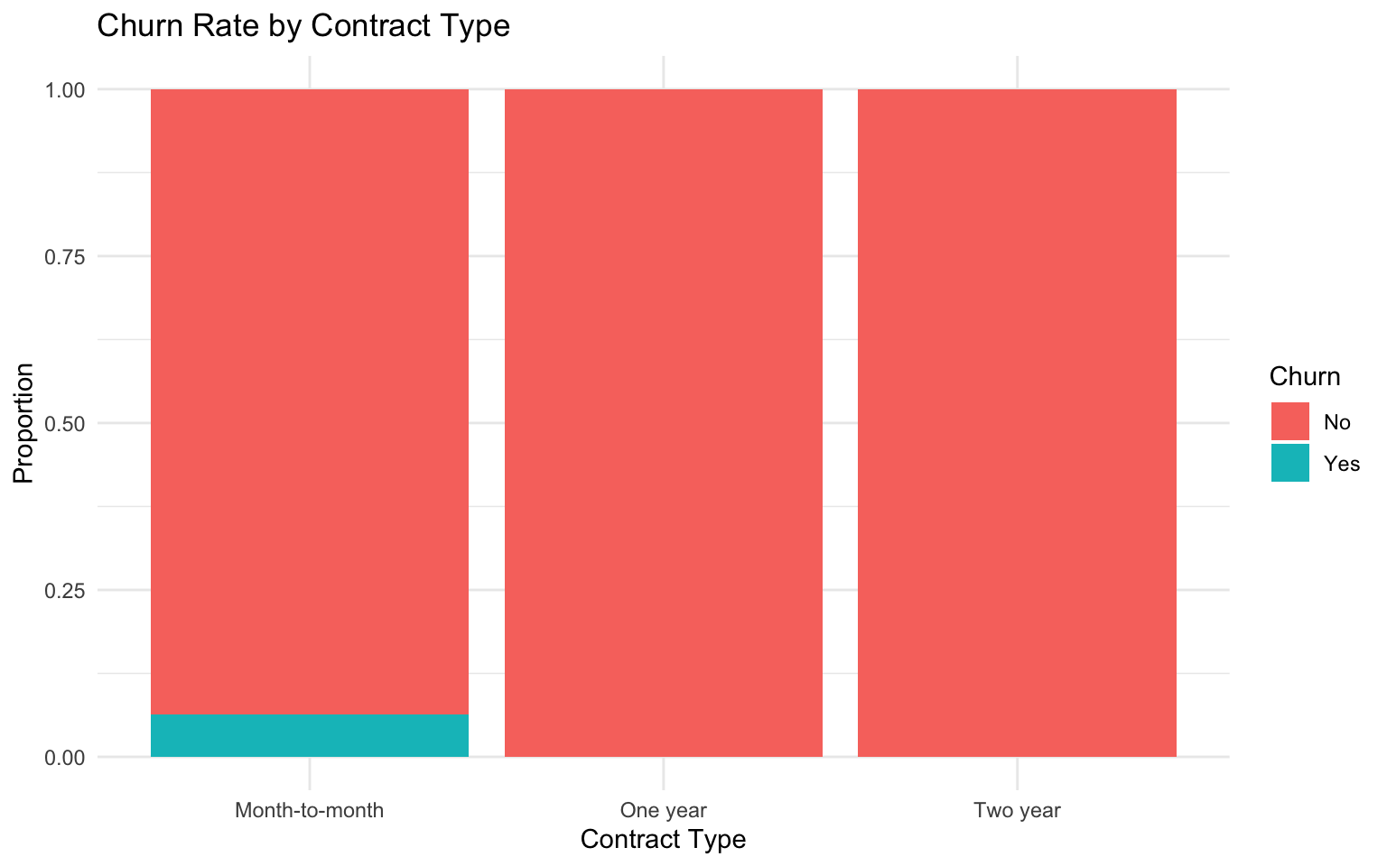
# Explore the relation between monthly charges and churn
ggplot(telecom_data, aes(x = monthly_charges, fill = churn)) +
  geom_histogram(position = "fill", bins = 30) +
  labs(
    title = "Churn Rate by Monthly Charges",
    x = "Monthly Charges",
    y = "Proportion",
    fill = "Churn"
  ) +
  theme_minimal()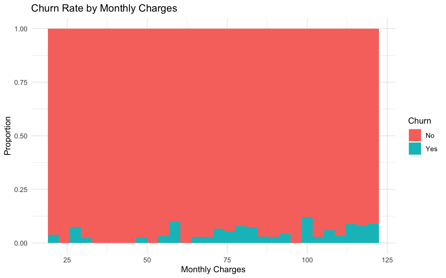
# Explore the relation between satisfaction score and churn
ggplot(telecom_data, aes(x = factor(satisfaction_score), fill = churn)) +
  geom_bar(position = "fill") +
  labs(
    title = "Churn Rate by Satisfaction Score",
    x = "Satisfaction Score",
    y = "Proportion",
    fill = "Churn"
  ) +
  theme_minimal()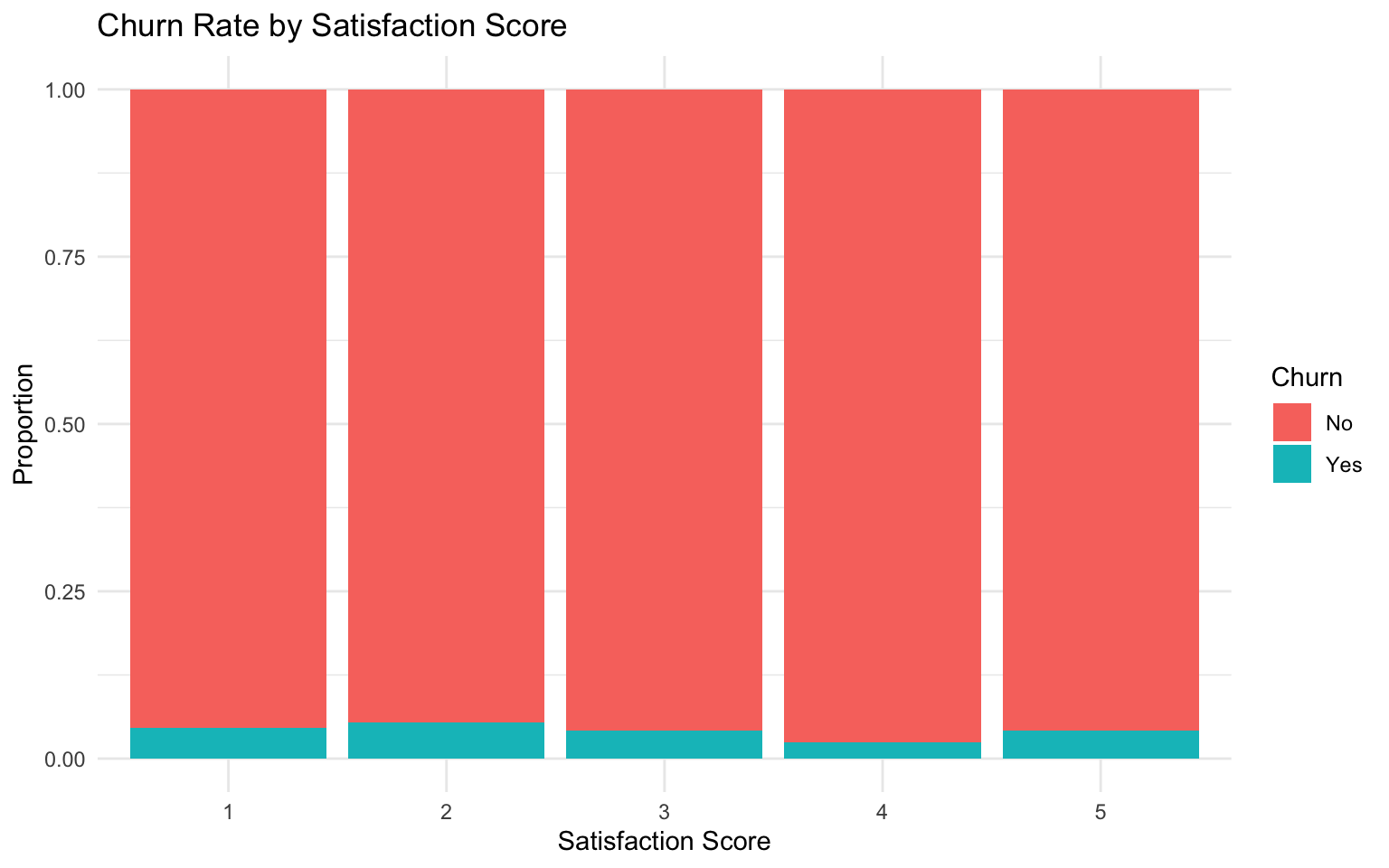
Data Preparation
Let’s prepare the data for modeling:
# Split the data into training and testing sets
set.seed(456)
telecom_split <- initial_split(telecom_data, prop = 0.75, strata = churn)
telecom_train <- training(telecom_split)
telecom_test <- testing(telecom_split)

# Create a recipe for preprocessing
telecom_recipe <- recipe(churn ~ tenure_months + contract + internet_service +
                         online_security + tech_support + monthly_charges +
                         satisfaction_score,
                        data = telecom_train) %>%
  step_dummy(all_nominal_predictors()) %>%
  step_normalize(all_numeric_predictors())

# Prepare the recipe
telecom_prep <- prep(telecom_recipe)

# Apply the recipe to the training and testing data
telecom_train_processed <- bake(telecom_prep, new_data = NULL)
telecom_test_processed <- bake(telecom_prep, new_data = telecom_test)
Model Building
Let’s build and compare several classification models:
# Fit a logistic regression model
logistic_model <- glm(churn ~ .,
                     data = telecom_train_processed,
                     family = "binomial")

# Fit a decision tree model
tree_model <- rpart(churn ~ .,
                   data = telecom_train_processed,
                   method = "class",
                   control = rpart.control(cp = 0.01))

# Fit a random forest model
rf_model <- ranger(
  formula = churn ~ .,
  data = telecom_train_processed,
  num.trees = 500,
  mtry = floor(sqrt(ncol(telecom_train_processed) - 1)),
  importance = "impurity",
  probability = TRUE
)
Model Evaluation
Let’s evaluate the performance of our models:
# Make predictions with logistic regression
logistic_pred <- telecom_test_processed %>%
  mutate(
    churn_prob = predict(logistic_model, newdata = telecom_test_processed, type = "response"),
    churn_pred = ifelse(churn_prob > 0.5, "Yes", "No"),
    churn_pred = factor(churn_pred, levels = c("No", "Yes"))
  )

# Make predictions with decision tree
tree_pred <- telecom_test_processed %>%
  mutate(
    churn_prob = predict(tree_model, newdata = telecom_test_processed, type = "prob")[, 2],
    churn_pred = predict(tree_model, newdata = telecom_test_processed, type = "class")
  )

# Make predictions with random forest
rf_pred <- telecom_test_processed %>%
  mutate(
    churn_prob = predict(rf_model, data = telecom_test_processed)$predictions[, 2],
    churn_pred = ifelse(churn_prob > 0.5, "Yes", "No"),
    churn_pred = factor(churn_pred, levels = c("No", "Yes"))
  )

# Combine predictions from all models
all_preds <- bind_rows(
  logistic_pred %>%
    select(churn, churn_prob, churn_pred) %>%
    mutate(model = "Logistic Regression"),
  tree_pred %>%
    select(churn, churn_prob, churn_pred) %>%
    mutate(model = "Decision Tree"),
  rf_pred %>%
    select(churn, churn_prob, churn_pred) %>%
    mutate(model = "Random Forest")
)

# Calculate metrics for all models
all_metrics <- all_preds %>%
  group_by(model) %>%
  summarize(
    accuracy = accuracy_vec(churn, churn_pred),
    precision = precision_vec(churn, churn_pred),
    recall = recall_vec(churn, churn_pred),
    f1 = f_meas_vec(churn, churn_pred),
    auc = roc_auc_vec(churn, churn_prob)
  )

# View the metrics
all_metrics
# A tibble: 3 × 6
model accuracy precision recall f1 auc
<chr> <dbl> <dbl> <dbl> <dbl> <dbl>
1 Decision Tree 0.96 0.96 1 0.980 0.5
2 Logistic Regression 0.96 0.96 1 0.980 0.152
3 Random Forest 0.96 0.96 1 0.980 0.313# Create ROC curves for all models using pROC package
# Create a list to store ROC objects for each model
roc_list <- all_preds %>%
group_by(model) %>%
group_map(~roc(.x$churn, .x$churn_prob))Setting levels: control = No, case = YesSetting direction: controls < casesSetting levels: control = No, case = YesSetting direction: controls < casesSetting levels: control = No, case = YesSetting direction: controls < cases# Name the ROC objects in the list
names(roc_list) <- unique(all_preds$model)
# Calculate AUC for each model
auc_values <- sapply(roc_list, auc)
auc_labels <- paste0(names(auc_values), " (AUC = ", round(auc_values, 3), ")")
# Plot the ROC curves
ggroc(roc_list) +
geom_abline(slope = 1, intercept = 1, linetype = "dashed", color = "gray") +
scale_color_discrete(labels = auc_labels) +
labs(
title = "ROC Curves for Classification Models",
color = "Model"
) +
theme_minimal()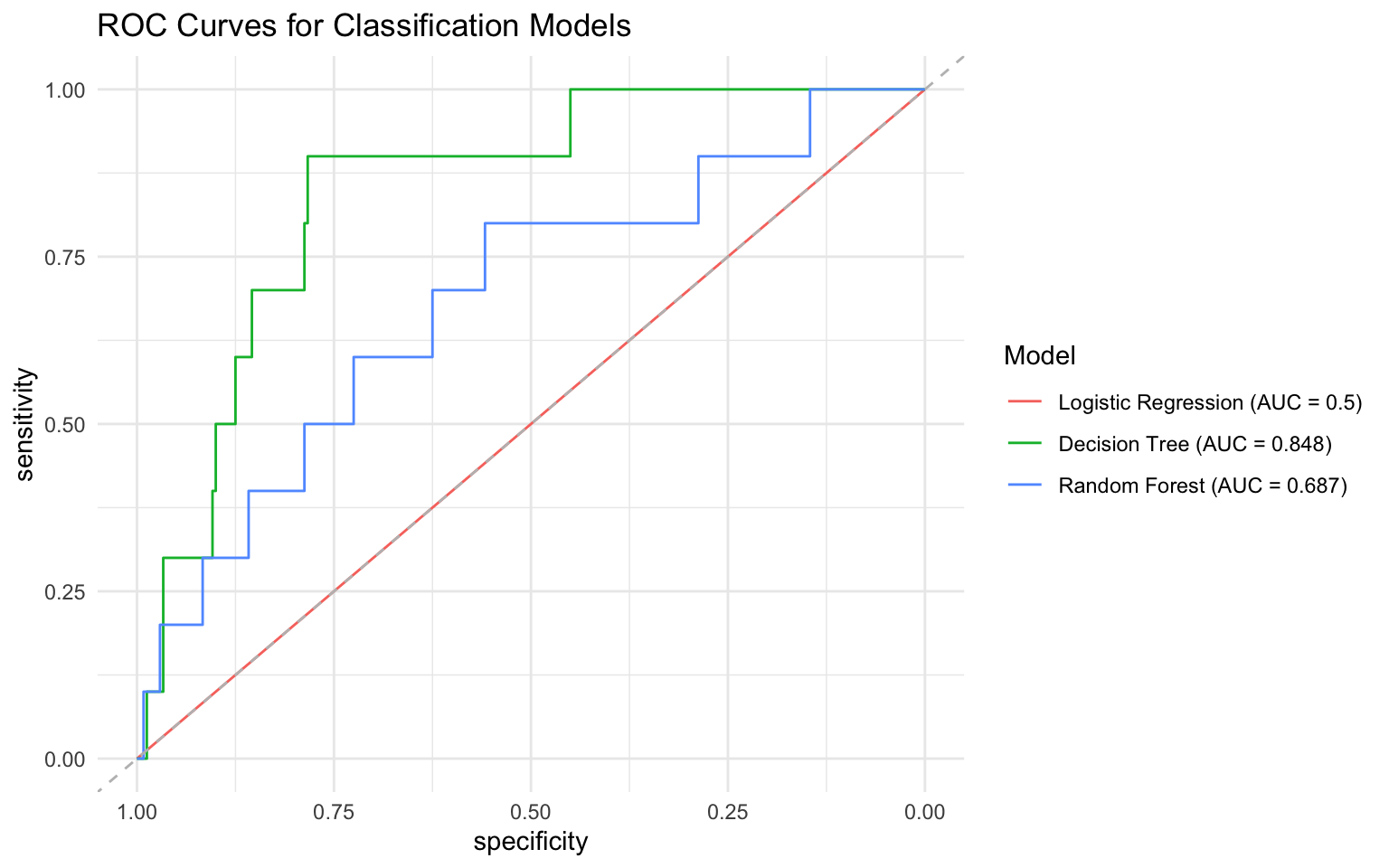
Variable Importance
Let’s examine which variables are most important for predicting churn:
# Extract variable importance from the random forest model
var_importance <- tibble(
  variable = names(importance(rf_model)),
  importance = importance(rf_model)
)

# Plot variable importance
ggplot(var_importance, aes(x = reorder(variable, importance), y = importance)) +
  geom_col() +
  coord_flip() +
  labs(
    title = "Variable Importance in Random Forest Model",
    x = NULL,
    y = "Importance"
  ) +
  theme_minimal()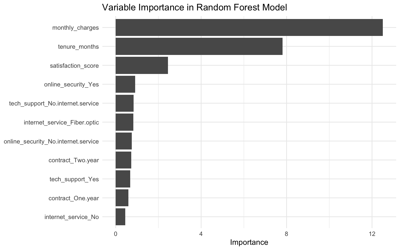
Customer Segmentation
We can use the predicted probabilities to segment customers into risk categories:
# Create risk segments
risk_segments <- rf_pred %>%
  mutate(
    risk_category = case_when(
      churn_prob < 0.3 ~ "Low Risk",
      churn_prob < 0.6 ~ "Medium Risk",
      TRUE ~ "High Risk"
    ),
    risk_category = factor(risk_category, levels = c("Low Risk", "Medium Risk", "High Risk"))
  )

# Count customers in each risk category
risk_segments %>%
  count(risk_category) %>%
  mutate(pct = n / sum(n) * 100)
# A tibble: 2 × 3
risk_category n pct
<fct> <int> <dbl>
1 Low Risk 248 99.2
2 Medium Risk 2 0.8# Visualize risk segments by contract type
ggplot(risk_segments, aes(x = risk_category, fill = telecom_test$contract)) +
geom_bar(position = "fill") +
labs(
title = "Risk Segments by Contract Type",
x = "Risk Category",
y = "Proportion",
fill = "Contract Type"
) +
theme_minimal()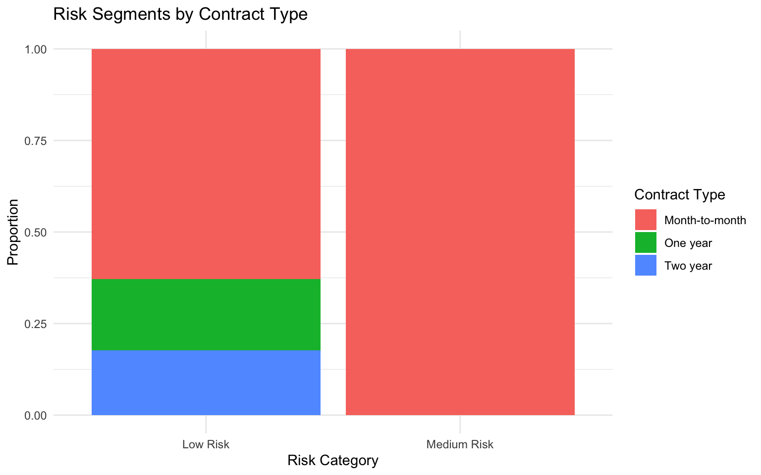
Business Recommendations
Based on our analysis, we can provide the following recommendations:
- Target High-Risk Customers: Focus retention efforts on customers identified as high-risk by the model.
- Contract Type: Encourage month-to-month customers to switch to longer-term contracts, which are associated with lower churn rates.
- Service Additions: Promote online security and tech support services, which are associated with lower churn rates.
- Customer Satisfaction: Implement programs to improve customer satisfaction, as higher satisfaction scores are associated with lower churn rates.
- Early Intervention: Develop special offers for customers in their first year of service, as churn rates are higher for customers with shorter tenure.
Implementation Plan
To implement the churn prediction model in a business setting:
- Automate Data Collection: Set up automated data pipelines to collect and preprocess customer data.
- Deploy the Model: Implement the random forest model in a production environment.
- Create a Dashboard: Develop a dashboard for the retention team to identify and track high-risk customers.
- Design Interventions: Create targeted retention offers based on customer characteristics and risk level.
- Monitor Performance: Continuously monitor the model’s performance and update it as needed.
4.10 Exercises
Exercise 1: Logistic Regression
Using the titanic dataset from the titanic package:
- Fit a logistic regression model to predict survival based on passenger characteristics.
- Interpret the coefficients in terms of odds ratios.
- Evaluate the model’s performance using appropriate metrics.
- Create visualizations to illustrate the relation between predictors and survival probability.
- Provide business recommendations based on your analysis.
Exercise 2: Decision Trees
Using a dataset of your choice:
- Fit a decision tree model for a classification problem.
- Visualize the decision tree and interpret the rules.
- Experiment with different values of the complexity parameter and observe the effect on the tree.
- Evaluate the model’s performance using appropriate metrics.
- Discuss the advantages and disadvantages of decision trees for your specific problem.
Exercise 3: Random Forests
Using the credit dataset from the ISLR package:
- Fit a random forest model to predict credit default.
- Examine variable importance and discuss which factors are most predictive of default.
- Tune the hyperparameters of the random forest (e.g.,
mtry,num.trees) to improve performance. - Compare the performance of the random forest to logistic regression and decision trees.
- Discuss the trade-offs between model complexity and interpretability.
Exercise 4: Business Application
You are a data scientist at an e-commerce company. You’ve been asked to develop a model to predict which customers are likely to make a purchase in the next 30 days:
- Create a simulated dataset with relevant features (e.g., browsing behavior, past purchases, demographics).
- Explore the relations in the data using appropriate visualizations.
- Fit multiple classification models and compare their performance.
- Handle any class imbalance issues.
- Provide business recommendations based on your analysis.
4.11 Summary
In this chapter, we’ve covered the fundamentals of classification for business applications. We’ve learned how to:
- Implement logistic regression models for binary classification
- Apply tree-based classification algorithms including decision trees and random forests
- Evaluate classification model performance using appropriate metrics
- Interpret classification results in business contexts
- Handle class imbalance in classification problems
- Compare and select models based on business requirements
- Visualize classification results for business presentations
These skills provide a solid foundation for predictive modeling in business contexts. By understanding how to predict categorical outcomes, you can make more informed business decisions and develop effective strategies for customer acquisition, retention, risk management, and more.
In the next chapter, we’ll build on these skills to explore model selection and hyperparameter tuning, which are essential for optimizing model performance.
4.12 References
- James, G., Witten, D., Hastie, T., & Tibshirani, R. (2021). An Introduction to Statistical Learning with Applications in R. Springer.
- Kuhn, M., & Johnson, K. (2013). Applied Predictive Modeling. Springer.
- Breiman, L. (2001). Random Forests. Machine Learning, 45(1), 5-32.
- Hosmer, D. W., Lemeshow, S., & Sturdivant, R. X. (2013). Applied Logistic Regression. Wiley.
- Kuhn, M., & Silge, J. (2022). Tidy Modeling with R. O’Reilly Media. https://www.tmwr.org/